| CSVS & State Condition1 | CSVS & State Condition2 | Correlation | P_Value | Correlation Direction | Statistically Significant | Practically Significant |
|---|---|---|---|---|---|---|
| CKD_rate | COPD_rate | 0.7015814 | 0.0000000 | ↑ | Yes | Yes |
| CKD_rate | CVD_rate | 0.6857228 | 0.0000000 | ↑ | Yes | Yes |
| CKD_rate | HghRskOB_rate | 0.9197652 | 0.0000000 | ↑ | Yes | Yes |
| CKD_rate | LBW_rate | 0.8027499 | 0.0000000 | ↑ | Yes | Yes |
| CKD_rate | LIPID_rate | 0.1380761 | 0.0429640 | ↑ | Yes | No |
| CKD_rate | OBESITY_rate | 0.1270219 | 0.0489740 | ↑ | Yes | No |
| CKD_rate | PM2_5 | -0.1712646 | 0.0017917 | ↓ | Yes | No |
| CKD_rate | PSORIASIS_rate | 0.1598222 | 0.0050678 | ↑ | Yes | No |
| CKD_rate | Pesticides | 0.1982067 | 0.0004168 | ↑ | Yes | No |
| CKD_rate | Pollution | -0.0456261 | 0.0251356 | ↓ | Yes | No |
| CKD_rate | PollutionScore | -0.0456261 | 0.0251356 | ↓ | Yes | No |
| CLD_rate | Parkinson_rate | 0.9432960 | 0.0000000 | ↑ | Yes | Yes |
| COPD_rate | CVD_rate | 0.9341342 | 0.0000000 | ↑ | Yes | Yes |
| COPD_rate | HghRskOB_rate | 0.6531102 | 0.0000000 | ↑ | Yes | Yes |
| COPD_rate | LBW_rate | 0.5595983 | 0.0000000 | ↑ | Yes | Yes |
| COPD_rate | LIPID_rate | 0.1348358 | 0.0450249 | ↑ | Yes | No |
| COPD_rate | Ozone | -0.1074270 | 0.0303209 | ↓ | Yes | No |
| COPD_rate | PM2_5 | -0.1825432 | 0.0007374 | ↓ | Yes | No |
| COPD_rate | PSORIASIS_rate | 0.1988266 | 0.0018043 | ↑ | Yes | No |
| COPD_rate | Pesticides | 0.2311310 | 0.0001675 | ↑ | Yes | No |
| COPD_rate | Pollution | -0.0315621 | 0.0182577 | ↓ | Yes | No |
| COPD_rate | PollutionScore | -0.0315621 | 0.0182577 | ↓ | Yes | No |
| CVD_rate | HghRskOB_rate | 0.6437518 | 0.0000000 | ↑ | Yes | Yes |
| CVD_rate | LBW_rate | 0.5143918 | 0.0000000 | ↑ | Yes | Yes |
| CVD_rate | LIPID_rate | 0.1445545 | 0.0381668 | ↑ | Yes | No |
| CVD_rate | OBESITY_rate | 0.1259491 | 0.0482050 | ↑ | Yes | No |
| CVD_rate | Ozone | -0.1132039 | 0.0297410 | ↓ | Yes | No |
| CVD_rate | PM2_5 | -0.1927883 | 0.0007421 | ↓ | Yes | No |
| CVD_rate | PSORIASIS_rate | 0.2042724 | 0.0016682 | ↑ | Yes | No |
| CVD_rate | Pesticides | 0.2553823 | 0.0000980 | ↑ | Yes | No |
| CVD_rate | Pollution | -0.0326592 | 0.0196896 | ↓ | Yes | No |
| CVD_rate | PollutionScore | -0.0326592 | 0.0196896 | ↓ | Yes | No |
| ChrDs_rate | CLD_rate | 0.2085732 | 0.0143378 | ↑ | Yes | No |
| ChrDs_rate | HTN_rate | 0.3783198 | 0.0000105 | ↑ | Yes | No |
| ChrDs_rate | LIPID_rate | 0.3406696 | 0.0000190 | ↑ | Yes | No |
| ChrDs_rate | OBESITY_rate | 0.1965699 | 0.0033693 | ↑ | Yes | No |
| ChrDs_rate | Parkinson_rate | 0.2183232 | 0.0146606 | ↑ | Yes | No |
| Cleanups | HTN_rate | -0.0361357 | 0.0471897 | ↓ | Yes | No |
| DM_rate | HTN_rate | 0.3170321 | 0.0000158 | ↑ | Yes | No |
| DM_rate | LIPID_rate | 0.3314622 | 0.0002440 | ↑ | Yes | No |
| DM_rate | Pollution | -0.0839124 | 0.0308810 | ↓ | Yes | No |
| DM_rate | PollutionScore | -0.0839124 | 0.0308810 | ↓ | Yes | No |
| DM_rate | ThyroidDs_rate | 0.5380157 | 0.0000000 | ↑ | Yes | Yes |
| HTN_rate | LIPID_rate | 0.2435055 | 0.0001208 | ↑ | Yes | No |
| HTN_rate | OBESITY_rate | 0.2157563 | 0.0039644 | ↑ | Yes | No |
| HTN_rate | ThyroidDs_rate | 0.3261153 | 0.0000269 | ↑ | Yes | No |
| HghRskOB_rate | LBW_rate | 0.9158799 | 0.0000000 | ↑ | Yes | Yes |
| HghRskOB_rate | LIPID_rate | 0.1473643 | 0.0397802 | ↑ | Yes | No |
| HghRskOB_rate | OBESITY_rate | 0.1333590 | 0.0463762 | ↑ | Yes | No |
| HghRskOB_rate | PM2_5 | -0.1781355 | 0.0017170 | ↓ | Yes | No |
| HghRskOB_rate | PSORIASIS_rate | 0.1639050 | 0.0055791 | ↑ | Yes | No |
| HghRskOB_rate | Pesticides | 0.2200658 | 0.0003210 | ↑ | Yes | No |
| HghRskOB_rate | Pollution | -0.0417125 | 0.0256512 | ↓ | Yes | No |
| HghRskOB_rate | PollutionScore | -0.0417125 | 0.0256512 | ↓ | Yes | No |
| LBW_rate | LIPID_rate | 0.1313685 | 0.0461943 | ↑ | Yes | No |
| LBW_rate | OBESITY_rate | 0.1259201 | 0.0492684 | ↑ | Yes | No |
| LBW_rate | PM2_5 | -0.1590149 | 0.0017496 | ↓ | Yes | No |
| LBW_rate | PSORIASIS_rate | 0.1303952 | 0.0090871 | ↑ | Yes | No |
| LBW_rate | Pesticides | 0.2020137 | 0.0004672 | ↑ | Yes | No |
| LBW_rate | Pollution | -0.0376904 | 0.0240200 | ↓ | Yes | No |
| LBW_rate | PollutionScore | -0.0376904 | 0.0240200 | ↓ | Yes | No |
| LIPID_rate | OBESITY_rate | 0.2510721 | 0.0002955 | ↑ | Yes | No |
| LIPID_rate | PM2_5 | -0.0941291 | 0.0284901 | ↓ | Yes | No |
| LIPID_rate | Pollution | -0.0303585 | 0.0378697 | ↓ | Yes | No |
| LIPID_rate | PollutionScore | -0.0303585 | 0.0378697 | ↓ | Yes | No |
| OBESITY_rate | Pollution | -0.0399506 | 0.0423155 | ↓ | Yes | No |
| OBESITY_rate | PollutionScore | -0.0399506 | 0.0423155 | ↓ | Yes | No |
| PM2_5 | PSORIASIS_rate | -0.0770409 | 0.0274381 | ↓ | Yes | No |
| Pollution | ThyroidDs_rate | -0.0590682 | 0.0453837 | ↓ | Yes | No |
| PollutionScore | ThyroidDs_rate | -0.0590682 | 0.0453837 | ↓ | Yes | No |
An Overview of the Relationship Between Environmental and Social Factors on select Diseases at CSVS
A Report on CSVS select diseases Utilizing CalEnviroScreen
Goal
- Assess CSVS Chronic disease rates and obstetric outcomes within the context of CA environmental factors
- Provide CSVS and other stakeholders with actionable insights.
- Provide groundwork for future research.
Introduction
Chronic diseases and obstetric outcomes are intertwined with social and environmental factors that impact health disparities. Clinica de Salud del Valle de Salinas (CSVS) delivers essential healthcare services to underserved, farmworker families and other demographic groups in the state of California.
The CalEnviroScreen (https://oehha.ca.gov/calenviroscreen/report/calenviroscreen-40) is a screening methodology that can be used to help identify California communities that are disproportionately burdened by multiple sources of pollution and social determinants of health.
By applying the same methodology to select clinical conditions (chronic diseases and OB outcomes) at CSVS, we hope to identify similarly impacted communities and detect the relationship between the diseases and pollutants.
CA Environmental Screen Dictionary
Methodology
This analysis was conducted to explore the relationship between chronic diseases, obstetric outcomes, and environmental factors in the service area of CSVS. The methodology employed is detailed below:
Study Design
This report utilized a cross-sectional design to analyze data collected during the period from 2022-2024.
The analysis focused on identifying correlations between health outcomes (chronic diseases and obstetric outcomes) and environmental and social determinants of health, as captured by the CalEnviroScreen tool.
Data Sources
- Health Outcome Data:
- Chronic disease rates were obtained from CSVS records in the EHR (Next-Gen) and then, standardized for population differences and adjusted for age.
- Health outcomes data included rates of conditions such as:
- Hypertension (HTN),
- Asthma
- Obesity
- Lipid Disorders
- Thyroid Diseases
- Gastroesophageal Reflux Disease (GERD)
- Type 2 Diabetes Mellitus (DM)
- Cardiovascular Disease (CVD)
- Chronic Liver Disease (CLD)
- Chronic Obstructive Pulmonary Disease (COPD)
- Psoriasis
- Chronic Kidney Disease (CKD)
- Parkinson’s Disease
- Chronic Diseases (ChrDs)
- The OB data was obtained from Natividad Hospital’s OB delivery records for CSVS patients analyzed subsequently at CSVS:
- Low Birth Weight (LBW)
- High-Risk Pregnancy (HghRskOB).
- Health outcomes data included rates of conditions such as:
- Chronic disease rates were obtained from CSVS records in the EHR (Next-Gen) and then, standardized for population differences and adjusted for age.
- Environmental Data:
- Environmental and socioeconomic data were sourced from the CalEnviroScreen tool (https://oehha.ca.gov/calenviroscreen/report/calenviroscreen-40), which provides region-specific scores, rates and percentiles across ZIP codes in the study area.
Data Preparation
Health outcome data from CSVS were analysed using standard population adjustment methods based on California Census 2020 population report.
Age adjustments were performed using standard age adjustment based on a California Census 2020 population report.
CA Environmental data were harmonized with CSVS health outcome data by matching ZIP codes and geographic boundaries.
Variables and Measures
Independent Variables: Environmental factors such as PM2.5, ozone levels, pesticide exposure, and socioeconomic indicators (e.g., poverty, unemployment); low birth weight, Hypertension, etc
Dependent Variables: Population-standardized and age-adjusted rates of chronic diseases and obstetric outcomes and percentiles.
- For population standardization LBW and High Risk Pregnancy, female populations were used as denominator
Covariates: Socioeconomic factors (e.g., education level, linguistic isolation) were considered as potential confounders.
Statistical Analysis
- Descriptive Statistics: Summary statistics were generated to describe the distribution of health outcomes and environmental factors across the study area.
- Correlation Analysis: Pearson and Spearman correlation coefficients were calculated to examine relationships between environmental factors and health outcomes. Statistical significance was assessed at p < 0.05.
- Spatial Analysis:
- Moran’s I and Geary’s C were calculated to assess the spatial autocorrelation of health outcomes and environmental factors.
- Local Indicators of Spatial Association (LISA) were used to identify hotspots and clusters.
- Visualization: Correlation matrices and spatial maps were generated to illustrate relationships and geographic patterns.
Software and Tools
Data cleaning and processing, statistical analyses, and visualization were performed using R (version 4.4.0) with the following packages:
Data manipulation: dplyr, tidyr, janitor and others
Statistical analysis: corrplot, sf, epitools
Spatial analysis: spdep, sf, lisa and others
Visualization: ggplot2, leaflet, mapview
Interactive graphics: Shiny
Report (this document): quarto
Limitations
The analysis was limited to data collected within 2 years, which may not capture long-term trends.
Some variables may be underrepresented in the available datasets. For instance, the pesticide indicator covers 132 active pesticide ingredients used in production agriculture, but lacks data on non-production and non-agricultural pesticide use, which is available only at the county level.
The active patients in the CSVS do not represent the entire county; they are a small subset from their respective zip codes.
The states only report disease counts greater than 12 for statistical purposes. Since our numbers are lower, we used all counts, including those below 12.
To gain a better understanding by comparing individual-level data with community-level data, we need to run a multi-level fixed effects model. This model will include a within-person effect for individuals and a separate effect for areas (zip codes). Additionally, we may consider using a count-based model, such as Poisson, and potentially a zero-inflated model if our outcomes exhibit a skewed distribution with a low skew.
RESULTS
Example MAPS
Mapping by Zipcode the rates of some select chronic diseases. Mapping is also available by percentile distribution by zipcode for each condition
<Link to Shiny App URL, app.R>
1. Correlations
2. Spatial Analysis
Here we analyze a different type of relationship – the spatial distribution and spatial profile of each condition or variable using zip codes as spatial units. We aim to answer the question:
- does the condition or variable form clustering patterns among the zip codes or is it dispersed?
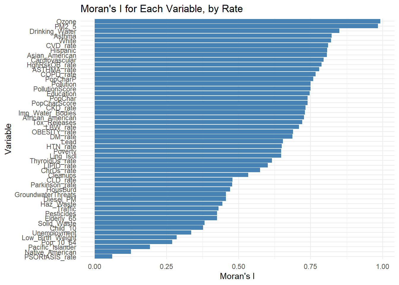
Moran’s I for Each Variable
Assess clustering tendency of conditions
Moran’s I measures Local spatial autocorrelation, revealing how strongly variables cluster across regions.
Environmental factors like ozone and PM2.5 have the highest Moran’s I values, suggesting strong global clustering, likely driven by shared geographic or industrial factors.
In contrast, variables like psoriasis and Native American population distribution exhibit low Moran’s I values, indicating more spatial randomness.
These findings underscore the need for targeted spatial interventions for environmental risks.
For example, high Moran’s I values for air quality variables suggest a need for regional air pollution control strategies, while conditions like psoriasis may require non-geographic approaches focusing on broader population health management.
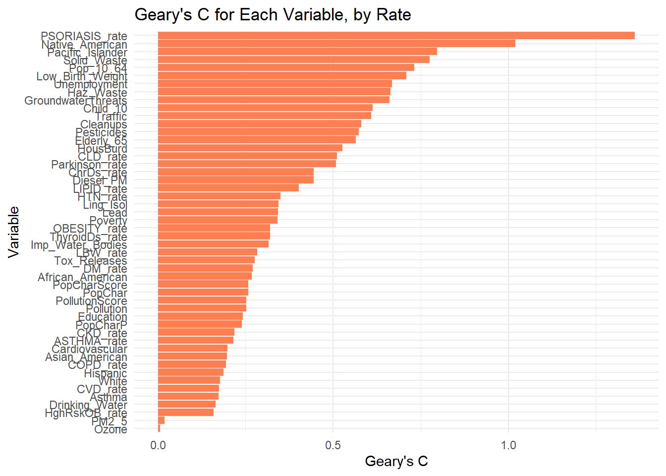
Geary’s C for Each Variable
Assess dispersal tendency of conditions
Geary’s C, on the other hand, measures negative spatial autocorrelation, which means “dispersal” tendency, with higher values indicating stronger dispersal.
variables such as Psoriasis, Native American population and Pacific Islander exhibit higher Geary’s C values in their distribution, indicating more spatial randomness (dispersal) and less localized clustering.
variables like ozone levels and PM2.5 and High Risk OB exhibit have the lowest Geary’s C value, indicting weak dispersal tendency, equivalent to strong local clustering distribution
These findings emphasize the importance of spatial targeting in public health and environmental interventions.
For instance, policies to mitigate air pollution should focus on identified hotspots, while addressing conditions like psoriasis may require more distributed, population-wide approaches.
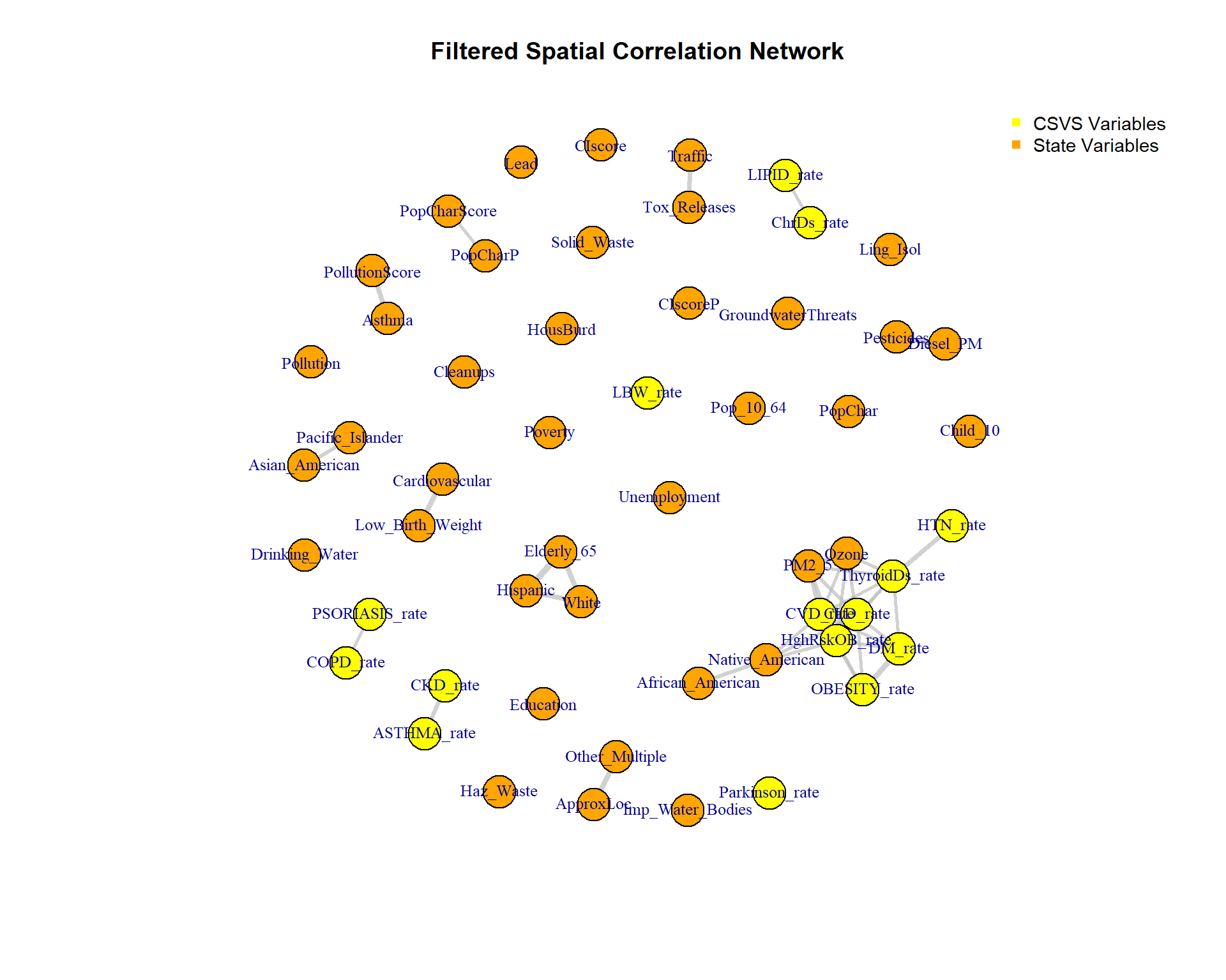
Combined Moran’s I and Geary’s C
Comparing Spatial Distribution
While the above analyzes spatial correlation, this section, which features a Network plot, with connecting lines indicating a closely matching relationship, will compare the spatial appearance of the conditions across zipcodes among themselves, thus to answer the question:
- when mapped, do the spatial patterns match (resemblance), where, for example, a complete overlap when overlaid would be a perfect score?
From the plot, we may make the following broad conclusions:
- spatial pattern matching is more likely mostly among the state variables as a group or among CSVS variables as a group, without much cross-matching
- matching variables in either major group contain mostly 2 elements; just one has 3 elements.
- the exception is one match with 7 CSVS variables and 4 State variables
- the implication with this 11-element cluster is that State variables like African American, Native American, PM2 and Ozone spatial distribution may coincide with CSVS Obesity, DM, CVD, CLD, High Risk OB, Thyroid Disease, and HTN distribution.
What does the map look like for these significantly closely matched conditions?
Comparing CSVS Vs State conditions
In the next section, we will compare the rates and distribution of the only clinical conditions included by the State with CSVS data: Low Birth Weight, Asthma, and Cardiovascular Disease
5. Summary of Results
Younger Population Health: The prevalence of asthma, obesity, and high-risk pregnancies reflects the clinic’s younger Latino farmworker population.
ZIP Code Priorities:
Greenfield (93927): High LBW rates and environmental risks require urgent maternal health and environmental interventions. CITED FROM WHERE WE GOT THE RESULT
Salinas (93905, 93906): Elevated rates of LBW, CVD, and asthma highlight overlapping health risks. CITED FROM WHERE WE GOT THE RESULT AND LARGEST NUMBERS, DENSE POPULATION
Environmental Risks: Air pollution, pesticide exposure, and poor living conditions exacerbate respiratory and cardiovascular burdens in farmworking communities. For our population we couldnt find it menaninful, even when among the state they are.
Health Co-Occurrences: Obesity, diabetes, and high-risk pregnancy are interconnected issues requiring integrated prevention programs
Consistency between the Correlations, Co-occurrence, and Spatial Patterns that Ozone and PM 2.5 are the environmental factors more related to Chronic disease among CSVS Patients.
6. Recommendations
- Health Screening and Management Programs:
- Prioritize cardiovascular, asthma, and chronic disease screenings in ZIP codes with elevated rates, particularly 93933 (Marina) and 93905/93906 (Salinas).
- Maternal and Child Health Services:
- Enhance prenatal care and education programs in Greenfield and Salinas to reduce LBW rates and improve maternal outcomes. Explain that this conditation may play a role even when there was not statistical significance.
- Environmental Health Initiatives:
- Mitigate air pollution and pesticide exposure in Greenfield and surrounding areas to reduce respiratory and cardiovascular risks. I can mention that the main source of pollution is traffic(use of personal cars).
- Community Outreach Programs:
- Tailor health initiatives to serve aging populations, addressing cultural and demographic needs.
- Geographic Resource Allocation:
- Use spatial clustering insights to prioritize healthcare resources in high-burden areas, focusing on ZIP codes with overlapping health and environmental challenges.
These targeted efforts will allow CSVS to address systemic health disparities, improve population health outcomes, and create sustainable changes in the community.
7. Conclusion
This analysis and presentation
- show our capability to deploy State Data tools and Statistical methods to generate disease rates and percentiles in CSVS geographic area of operation
- allow us to compare rates between and among different variables, State Vs CSVS, or within each camp
- demonstrate our ability to determine correlations in rates and percentiles across and within camps
- facilitate spatial correlations enabling overlap comparisons among all variables, State or CSVS