---
title: "CSVS OB DATA Analytics"
author: "Oguchi Nkwocha, MD., MS."
format:
html:
page-layout: full
code-tools: true
toc: true
toc-depth: 6
number-sections: true
toc-location: left
theme: cosmo
comments:
hypothesis: true
---
```{r echo=FALSE, warning=FALSE, message=FALSE}
#setwd("C:/Users/onkwocha.CSVSLINK/Dropbox/OB_DATA")
library(readr)
library(openxlsx)
library(xlsx)
library(DataExplorer)
library(explore)
library(XICOR)
library(survival)
library(survminer)
library(klaR)
library(forestplot)
library(mice)
library(readxl)
library(dplyr)
library(purrr)
library(stringr)
library(randomForest)
library(leaflet)
library(sf)
library(tableone)
library(DT)
library(kableExtra)
library(tidyr)
#library(shiny)
library(quarto)
library(fastDummies)
library(downlit)
library(tidyverse)
library(magrittr)
library(ggplot2)
```
```{r echo=FALSE, warning=FALSE, message=FALSE}
ob_data_chr <- readRDS("Working OB Dataset.RDS")
ob_data_fctr <- readRDS("All Factored Complete Ready OB Dataset for Analytics.RDS")
```
# Introduction
OB service at CSVS is delivered by dedicated clinicians and staff who provide tools- and procedure-validated comprehensive natal education through the CPSP program; prenatal care, hospital and delivery care, as well as post-natal care. OB deliveries are currently performed only at NMC which keeps a standard meticulous record of the delivery event and related issues. Each phase of OB care --prenatal, peripartal and postpartal-- presents opportunities and challenges depending on the effects of relevant factors which impact care, especially the central event of OB care, Delivery.
The goal of this document is to explore the data and present analytical results for information, education and action where indicated.
# Overview
```{r echo=FALSE, warning=FALSE, message=FALSE}
ob_stats_block <- ob_data_chr
# Calculate days and months
library(lubridate)
# Define start and end dates
ob_data_orig <- readRDS("Base OB Data DB.RDS")
start_date <- min(ob_data_orig$adm_date)
end_date <- max(ob_data_orig$adm_date)
# Calculate the number of days
number_of_days <- as.numeric(end_date - start_date)
#print(paste("Number of days:", number_of_days))
# Calculate the number of months
date_interval <- lubridate::interval(start_date, end_date)
number_of_months <- time_length(date_interval, "months")
#print(paste("Number of months:", number_of_months))
# Other quick stats
dte_range_NMC_data <- range(ob_stats_block$adm_date)
del_tm_dur_range <- round(range((ob_stats_block$gest_age_days)/7),1)
age_range <- range(ob_stats_block$age)
nbr_del_nmc <- nrow(ob_stats_block)
prcnt_preterm <- round(sum(ob_stats_block$gest_age_days <259) / sum(ob_stats_block$gest_age_days >=140)*100,0)
gest_age_range <- range(ob_stats_block$gest_age_days, na.rm = TRUE)
prcnt_hghRsk <- round(sum(ob_stats_block$hghRsk=="yes")/nrow(ob_stats_block)*100,0)
mltpl_gest <- sum(ob_data_chr$baby_sq>1)
mltpl_gest_prcnt <- round(mltpl_gest/nrow(ob_data_chr)*100,1)
mltpl_gest_lvls <- levels(factor(ob_data_chr$baby_sq))
gndr <- table(ob_data_chr$gender)
gndr_prcnt <- round(prop.table(gndr)*100,1)
c_section <- sum(ob_stats_block$del_method_cnsldt!="Vaginal")
c_section_prcnt <- round(c_section / nrow(ob_stats_block)*100,1)
prim_c_section <- sum(ob_stats_block$del_method_cnsldt=="C/S, Primary")
#prim_c_section <- sum(ob_stats_block$del_method_cnsldt=="C/S, Primary")
prim_c_section_prcnt <- round(prim_c_section/nrow(ob_stats_block)*100, 1)
prim_c_section_prcnt_all.cs <- round(prim_c_section/c_section*100, 1)
repeat_cs_prcnt <- round(sum(ob_stats_block$delivery_method =="Repeat Cesarean Section")/nrow(ob_stats_block)*100, 1)
#Primip C/S with vertex presentation
primip_c_s <- ob_stats_block %>%
filter(grav ==1 & para ==0 & baby_sq == 1 & presentation == "Vertex" & str_detect(delivery_method, "Prim" ))
primip_prct_all_del <- round(nrow(primip_c_s)/nrow(ob_stats_block)*100,1)
primip_prct_all_c_section <- round(nrow(primip_c_s)/c_section*100, 1)
primip_prct_primary_c_section <- round(nrow(primip_c_s)/prim_c_section*100,1)
ave_daily_del <- round(nrow(ob_stats_block)/number_of_days,0)
ave_monthly_del <- round(nrow(ob_stats_block)/number_of_months,0)
ave_annual_del <- round(nrow(ob_stats_block)/9*4,0)
min_birth_wt <- min(ob_stats_block$weight[ob_stats_block$weight > 0])
max_birth_wt <- max(ob_stats_block$weight)
ave_birth_wt <- round(mean(ob_stats_block$weight[ob_stats_block$weight > 0],1))
sa_data <- nrow(ob_stats_block %>% filter(time >= 0))
sa_data_prcnt <- round(sa_data/nrow(ob_stats_block)*100,0)
```
Between `r dte_range_NMC_data[1]` and `r dte_range_NMC_data[2]`, a period of **9 quarters** or 27 months, ***`r nbr_del_nmc`*** CSVS prenatal patients delivered at NMC, which is the principal source of data for this analysis.This included **`r gndr[1]` females**, **`r gndr[2]` males** and **`r gndr[3]` unknowns** (`r gndr_prcnt[c(1:3)]` % respectively). There were **`r mltpl_gest` multiple gestations** --all twins -- a `r mltpl_gest_prcnt`% incidence. There was **1 Fetal Demise** during the period.
Primary Cesarean section rate was **```r prim_c_section_prcnt```%**, constituting **`r prim_c_section_prcnt_all.cs`%** of all c-sections. Repeat C-Section rate was **```r repeat_cs_prcnt```%**. Total C-section rate was **```r c_section_prcnt```%**.
_For **primip vertex** presentations_, the overall C-section rate is **```r primip_prct_all_del```%**. This accounts for **```r primip_prct_all_c_section```%** of all C-Sections, which is **```r primip_prct_primary_c_section```%** of all Primary Cesaerian Sections.
The average monthly delivery for CSVS for the period was **`r ave_monthly_del`**, with _annualized rate_ of **```r ave_annual_del```** deliveries. Each day, on the average, **`r ave_daily_del` deliveries** occurred.
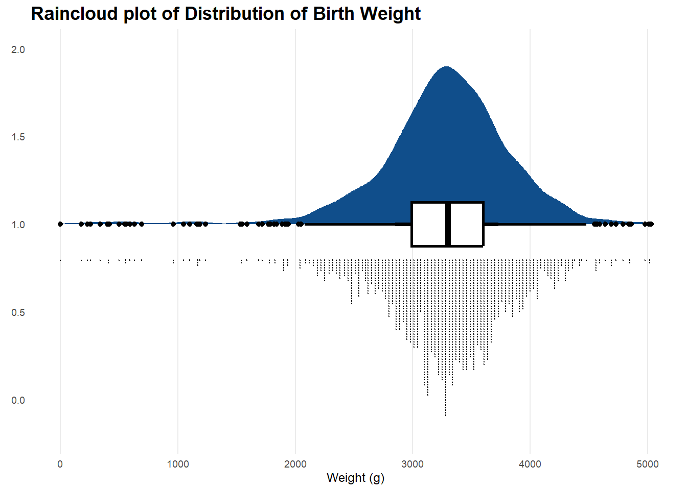
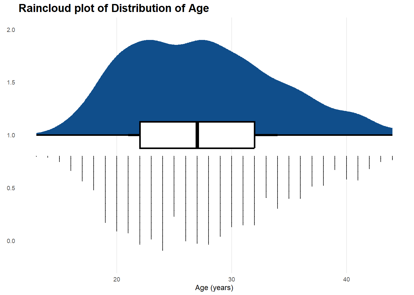
Average birth weight was **`r ave_birth_wt`gm**, with minimum **`r min_birth_wt`gm** and maximum of **`r max_birth_wt`gm**. Maternal age range was between ***`r age_range[1]`*** and ***`r age_range[2]`***, with a ***median age of `r median(ob_stats_block$age)`***. (See Histogram below)
## Exploring the Data
### Distributions and frequencies
```{r echo=FALSE, warning=FALSE, message=FALSE}
# Load necessary libraries
library(ggplot2)
library(ggdist)
library(dplyr)
# Function to create a raincloud plot
create_raincloud_plot <- function(data, variable, title, xlabel) {
ggplot2::ggplot(data, aes_string(x = variable, y = "1")) +
ggdist::stat_halfeye(fill = 'dodgerblue4') +
ggdist::stat_dots(
aes(y = 0.8),
fill = 'dodgerblue4',
color = 'black',
side = 'bottom'
) +
geom_boxplot(width = 0.25, color = 'black', linewidth = 1) +
theme_minimal(base_size = 9) +
labs(x = xlabel, y = element_blank(), title = title) +
theme(
panel.grid.minor = element_blank(),
panel.grid.major.y = element_blank(),
plot.title = element_text(size = rel(1.5), face = 'bold'),
legend.position = 'none'
) +
coord_cartesian(xlim = range(data[[variable]], na.rm = TRUE))
}
# Ensure columns are present and handle NA values
ob_data_chr_violin <- ob_data_chr %>%
dplyr::select(age, weight) %>%
na.omit()
# Create plots for age and weight
p1 <- create_raincloud_plot(ob_data_chr_violin, "age", "Raincloud plot of Distribution of Age", "Age (years)")
p2 <- create_raincloud_plot(ob_data_chr_violin, "weight", "Raincloud plot of Distribution of Birth Weight", "Weight (g)")
# Print plots
print(p2)
print(p1)
```
#### Other histograms
```{r echo=FALSE, message=FALSE, warning=FALSE}
#Gravity:
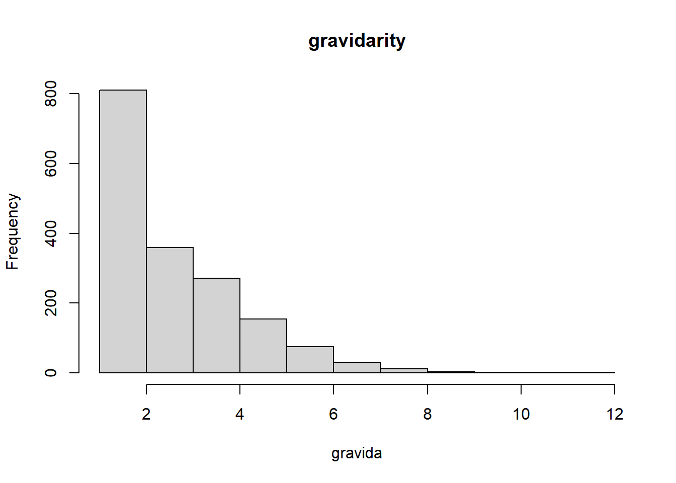
hist(ob_stats_block$grav, main = "gravidarity", xlab = "gravida")
#parity
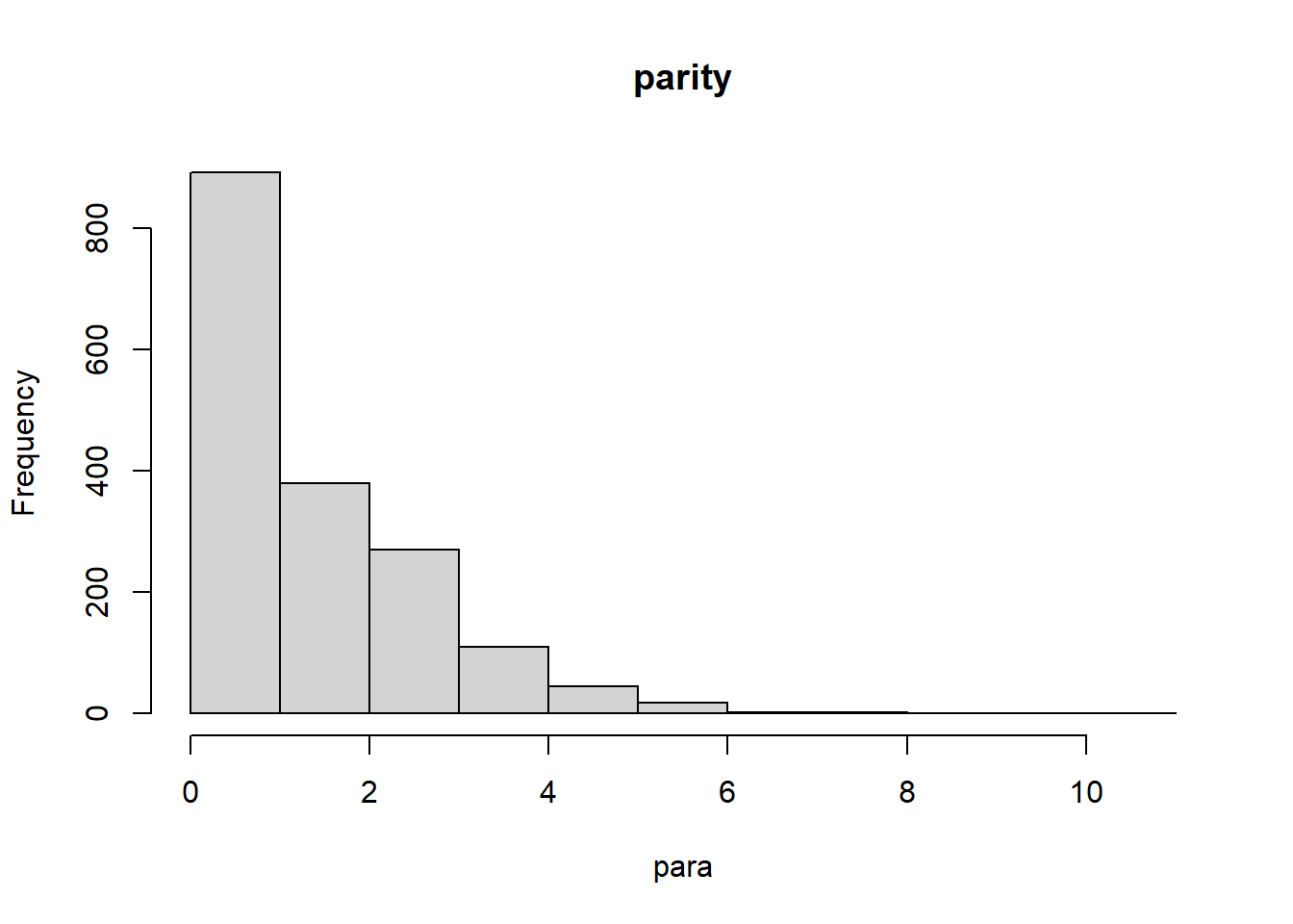
hist(ob_stats_block$para, main ="parity", xlab = "para")
#APGAR 1
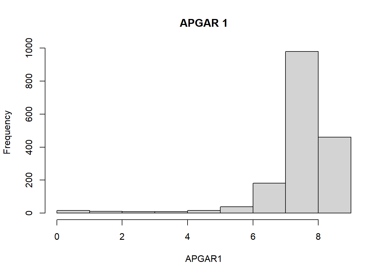
hist(ob_stats_block$apg1, main ="APGAR 1", xlab = "APGAR1")
#APGAR 2
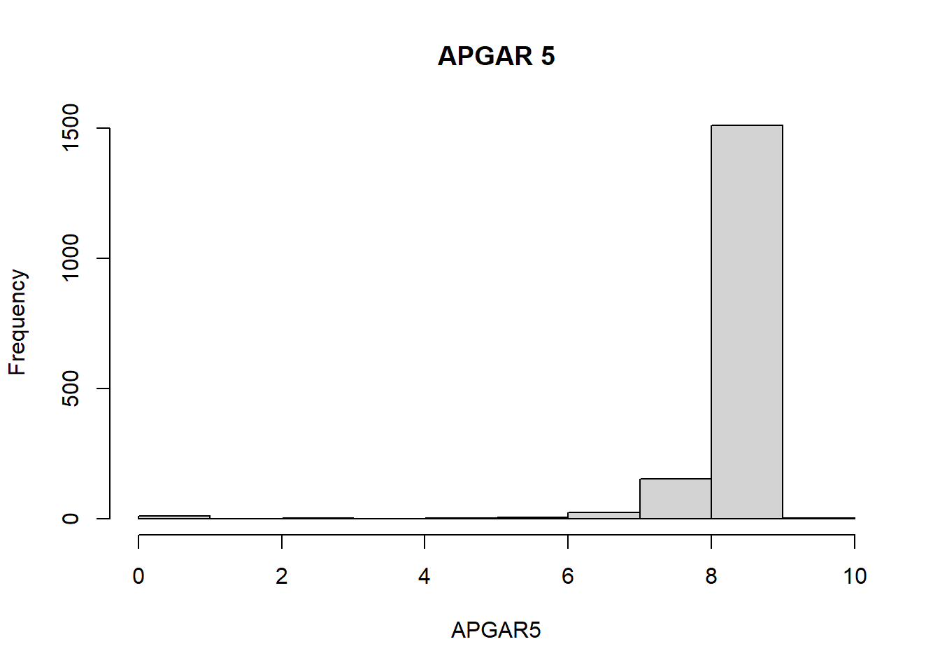
hist(ob_stats_block$apg5, main ="APGAR 5", xlab = "APGAR5")
```
```{r echo=FALSE, warning=FALSE, message=FALSE}
library(dplyr)
library(lubridate)
library(plotly)
library(ggplot2)
para_0_dta <- ob_stats_block %>%
filter(para ==0)
para_1_dta <- ob_stats_block %>%
filter(para ==1)
prcnt_p_0 <- round(nrow(para_0_dta)/nrow(ob_stats_block)*100,0)
prcnt_p_1 <- round(nrow(para_1_dta)/nrow(ob_stats_block)*100,0)
```
From the figures above, we learn that there
- relatively fewer pregnancies under age 19 than over 35
- primips account for **```r prcnt_p_0```%**; second pregnancies **```r prcnt_p_0```%**; so slightly over half of all our deliveries are to women with 1 or 2 deliveries, counting the current pregnancy as a delivery
- most deliveries score APGAR-1 8 and over; and APGAR-5 9
Does the Zip code make any difference with respect to gravidarity or parity?
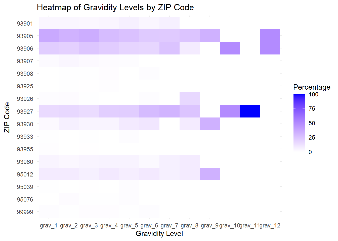
#### Gravidarity-Parity distribution by Zipcode
```{r echo=FALSE, warning=FALSE, message=FALSE}
ob_data_tbl_xtra <- readRDS("All Factored Complete Ready OB Dataset for Analytics.RDS") %>%
dplyr::select(-adm_date, -delivery_date) %>%
mutate(cluster = as.factor(cluster)) %>%
mutate(grav_fct = factor(grav),
para_fct = factor(para)) %>%
mutate(age_group = cut(age, breaks = c(-Inf, 21, 29, 35, Inf), labels = c("<21", "21-29", "29-35", ">35")),
age_group = factor(age_group))
##gravidarity
tmp <- tempfile()
sink(tmp)
strata_tbl_grav_zip <- CreateTableOne(data = ob_data_tbl_xtra, strata = "grav_fct", vars = "zip")
kableone(strata_tbl_grav_zip, cramVars = "grav_fct", caption = "Distribution of Gravidarity by Zip code")
sink()
# Remove the temporary file
unlink(tmp)
#Heat map to explain p-Value
library(stringr)
# Suppress print output by redirecting to a temporary file
tmp <- tempfile()
sink(tmp)
grav_zip_plt <- as.data.frame(print(strata_tbl_grav_zip, cramVars = "grav_fct"))
sink()
# Remove the temporary file
unlink(tmp)
# Verify that grav_zip_plt is now a data frame
#head(grav_zip_plt)
grav_zip_plt.hb <- grav_zip_plt %>%
slice(-1:-2) %>%
select(-p, -test)
# Clean and separate the percentages
cleaned_data <- grav_zip_plt.hb %>%
rownames_to_column(var = "zip") %>%
mutate(across(`1`:`12`, ~ str_extract(., "(?<=\\().+?(?=\\))"))) %>%
rename_with(~ paste0("grav_", 1:12), `1`:`12`)
# Reshape the data into long format
long_data <- cleaned_data %>%
pivot_longer(cols = starts_with("grav_"), names_to = "gravidity", values_to = "percent") %>%
mutate(percent = as.numeric(percent)) %>%
filter(!is.na(percent)) %>%
mutate(gravidity = factor(gravidity, levels = paste0("grav_", 1:12)))
# Create the heatmap plot
ggplot(long_data, aes(x = gravidity, y = zip, fill = percent)) +
geom_tile() +
labs(title = "Heatmap of Gravidity Levels by ZIP Code",
x = "Gravidity Level",
y = "ZIP Code",
fill = "Percentage") +
theme_minimal() +
scale_fill_gradient(low = "white", high = "blue", na.value = "grey50") +
scale_y_discrete(limits = rev(levels(as.factor(long_data$zip))))
##parity
strata_tbl_para_zip <- CreateTableOne(data = ob_data_tbl_xtra, strata = "para_fct", vars = "zip")
kableone(strata_tbl_para_zip, cramVars = "para_fct", caption = "Distribution of Parity by Zip code")
##parity -Zip heatmap
library(dplyr)
library(tidyr)
library(ggplot2)
library(stringr)
# Assuming para_zip_plt is your data frame
# Suppress print output by redirecting to a temporary file
tmp <- tempfile()
sink(tmp)
para_zip_plt <- as.data.frame(print(strata_tbl_para_zip, cramVars = "para_fct"))
sink()
# Remove the temporary file
unlink(tmp)
# Verify that grav_zip_plt is now a data frame
#head(grav_zip_plt)
para_zip_plt.hb <- para_zip_plt %>%
slice(-1:-2) %>%
select(-p, -test)
# Clean and separate the percentages
cleaned_data <- para_zip_plt.hb %>%
rownames_to_column(var = "zip") %>%
mutate(across(`0`:`9`, ~ str_extract(., "(?<=\\().+?(?=\\))"))) %>%
mutate(across(`11`, ~ str_extract(., "(?<=\\().+?(?=\\))"))) %>%
rename(para_0 = `0`, para_1 = `1`, para_2 = `2`, para_3 = `3`, para_4 = `4`,
para_5 = `5`, para_6 = `6`, para_7 = `7`, para_8 = `8`, para_9 = `9`,
para_11 = `11`)
# Reshape the data into long format
long_data <- cleaned_data %>%
pivot_longer(cols = starts_with("para_"), names_to = "parity", values_to = "percent") %>%
mutate(percent = as.numeric(percent)) %>%
filter(!is.na(percent)) %>%
mutate(parity = factor(parity, levels = paste0("para_", c(0:9, 11))))
# Create the heatmap plot
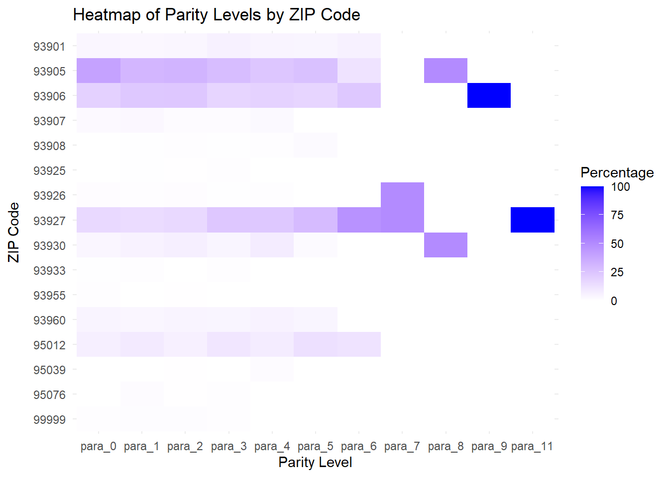
ggplot(long_data, aes(x = parity, y = zip, fill = percent)) +
geom_tile() +
labs(title = "Heatmap of Parity Levels by ZIP Code",
x = "Parity Level",
y = "ZIP Code",
fill = "Percentage") +
theme_minimal() +
scale_fill_gradient(low = "white", high = "blue", na.value = "grey50") +
scale_y_discrete(limits = rev(levels(as.factor(long_data$zip))))
```
Yes, there is a difference in the distribution, but only for Parity (number of deliveries) -- for both 93905 (higher in lower parity levels) and 93927 (higher in higher parity levels), with a significant p-value of 0.043. There was no difference with respect to Gravidarity (number of pregnancies)
Is there a difference in the distribution of different age-groups among and within zip codes? As before, first, check the p-value. It is 0.105, so the answer is, No.
#### Age categories distribution by zip
```{r echo=FALSE, message=FALSE, warning=FALSE}
strata_tbl_age_cat_para_zip <- CreateTableOne(data = ob_data_tbl_xtra, strata = "age_group", vars = "zip")
kableone(strata_tbl_age_cat_para_zip, caption = "Distribution of Age-groups by Zip Code")
# strata_tbl_age_cat_grav_zip <- CreateTableOne(data = ob_data_tbl_xtra, strata = "age_group", vars = "zip")
# kableone(strata_tbl_age_cat_grav_zip, cramVars = "grav_fct", caption = "Distribution of Age-groups by Gravidarity by Zip Code")
```
<!-- #### Age categories distribution by garavidarity-parity -->
<!-- ```{r echo=FALSE, message=FALSE, warning=FALSE} -->
<!-- strata_tbl_age_cat_para <- CreateTableOne(data = ob_data_tbl_xtra, strata = "age_group", vars = "para_fct") -->
<!-- kableone(strata_tbl_age_cat_para, cramVars = "age_group", caption = "Distribution of Age-groups by Parity") -->
<!-- strata_tbl_age_cat_grav <- CreateTableOne(data = ob_data_tbl_xtra, strata = "age_group", vars = "grav_fct") -->
<!-- kableone(strata_tbl_age_cat_grav, cramVars = "grav_fct", caption = "Distribution of Age-groups by Gravidarity") -->
<!-- ``` -->
#### Gravidarity-Parity distribution by Age
```{r echo=FALSE, warning=FALSE, message=FALSE}
# Load required libraries
library(dplyr)
library(ggplot2)
library(tableone)
library(knitr)
# Read data
ob_data_tbl_xtra <- readRDS("All Factored Complete Ready OB Dataset for Analytics.RDS") %>%
dplyr::select(-adm_date, -delivery_date) %>%
mutate(cluster = as.factor(cluster)) %>%
mutate(grav_fct = factor(grav), para_fct = factor(para)) %>%
mutate(age_group = cut(age, breaks = c(-Inf, 21, 29, 35, Inf), labels = c("<21", "21-29", "29-35", ">35")),
age_group = factor(age_group))
# Create table one
strata_tbl_age_cat_para <- CreateTableOne(data = ob_data_tbl_xtra, strata = "age_group", vars = "para_fct")
kableone(strata_tbl_age_cat_para, cramVars = "age_group", caption = "Distribution of Age-groups by Parity")
strata_tbl_age_cat_grav <- CreateTableOne(data = ob_data_tbl_xtra, strata = "age_group", vars = "grav_fct")
kableone(strata_tbl_age_cat_grav, cramVars = "grav_fct", caption = "Distribution of Age-groups by Gravidarity")
# Summarize data for plotting
plot_data_para <- ob_data_tbl_xtra %>%
group_by(age_group, para_fct) %>%
summarise(count = n()) %>%
ungroup() %>%
group_by(age_group) %>%
mutate(percentage = count / sum(count) * 100)
# Plot the distribution
ggplot(plot_data_para, aes(x = para_fct, y = percentage, fill = age_group)) +
geom_bar(stat = "identity", position = "dodge") +
geom_text(aes(label = sprintf("%.1f", percentage)),
position = position_dodge(width = 0.9), vjust = -0.5, size = 2) +
labs(title = "Distribution of Age-groups by Parity",
x = "Parity",
y = "Percentage",
fill = "Age Group") +
theme_minimal()
# Summarize data for plotting
plot_data <- ob_data_tbl_xtra %>%
group_by(age_group, para_fct) %>%
summarise(count = n()) %>%
ungroup() %>%
group_by(age_group) %>%
mutate(percentage = count / sum(count) * 100) %>%
mutate(para_fct = as.numeric(as.character(para_fct))) %>%
arrange(age_group, para_fct)
# Plot the distribution with lines and area shading
ggplot(plot_data, aes(x = para_fct, y = percentage, color = age_group, fill = age_group)) +
geom_line(size = 1) +
geom_ribbon(aes(ymin = 0, ymax = percentage), alpha = 0.3) +
labs(title = "Distribution of Age-groups by Parity",
x = "Parity",
y = "Percentage",
fill = "Age Group",
color = "Age Group") +
scale_x_continuous(breaks = seq(min(plot_data$para_fct), max(plot_data$para_fct), by = 2)) +
theme_minimal()
# Summarize data for plotting
plot_data_grav <- ob_data_tbl_xtra %>%
group_by(age_group, grav_fct) %>%
summarise(count = n()) %>%
ungroup() %>%
group_by(age_group) %>%
mutate(percentage = count / sum(count) * 100)
# Plot the distribution
ggplot(plot_data_grav, aes(x = grav_fct, y = percentage, fill = age_group)) +
geom_bar(stat = "identity", position = "dodge") +
geom_text(aes(label = sprintf("%.1f", percentage)),
position = position_dodge(width = 0.9), vjust = -0.5, size = 2) +
labs(title = "Distribution of Age-groups by Gravidarity",
x = "Gravidarity",
y = "Percentage",
fill = "Age Group") +
theme_minimal()
# Summarize data for plotting
plot_data <- ob_data_tbl_xtra %>%
group_by(age_group, grav_fct) %>%
summarise(count = n()) %>%
ungroup() %>%
group_by(age_group) %>%
mutate(percentage = count / sum(count) * 100) %>%
mutate(grav_fct = as.numeric(as.character(grav_fct))) %>%
arrange(age_group, grav_fct)
# Plot the distribution with lines and area shading
ggplot(plot_data, aes(x = grav_fct, y = percentage, color = age_group, fill = age_group)) +
geom_line(size = 1) +
geom_ribbon(aes(ymin = 0, ymax = percentage), alpha = 0.3) +
labs(title = "Distribution of Age-groups by Gravidarity",
x = "Gravidarity",
y = "Percentage",
fill = "Age Group",
color = "Age Group") +
scale_x_continuous(breaks = seq(min(plot_data$grav_fct), max(plot_data$grav_fct), by = 2)) +
theme_minimal()
```
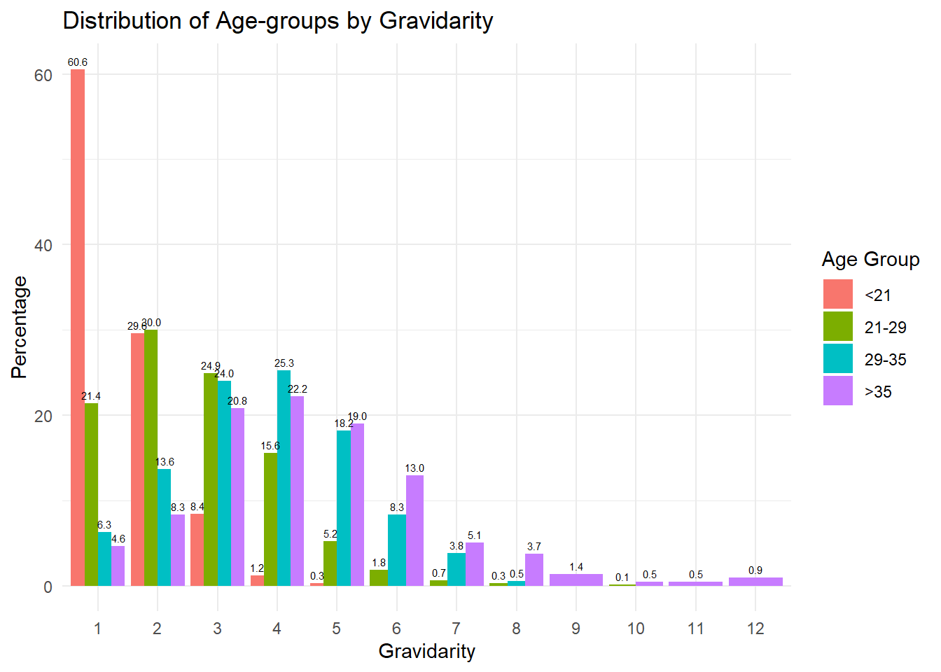
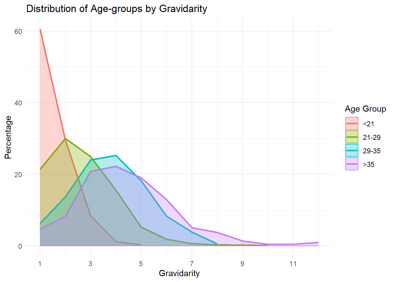
Yes, there is a significant difference (p = <0.001 for both) in the distribution of _Gravidarity_ and of _Parity_ within and among zip codes.
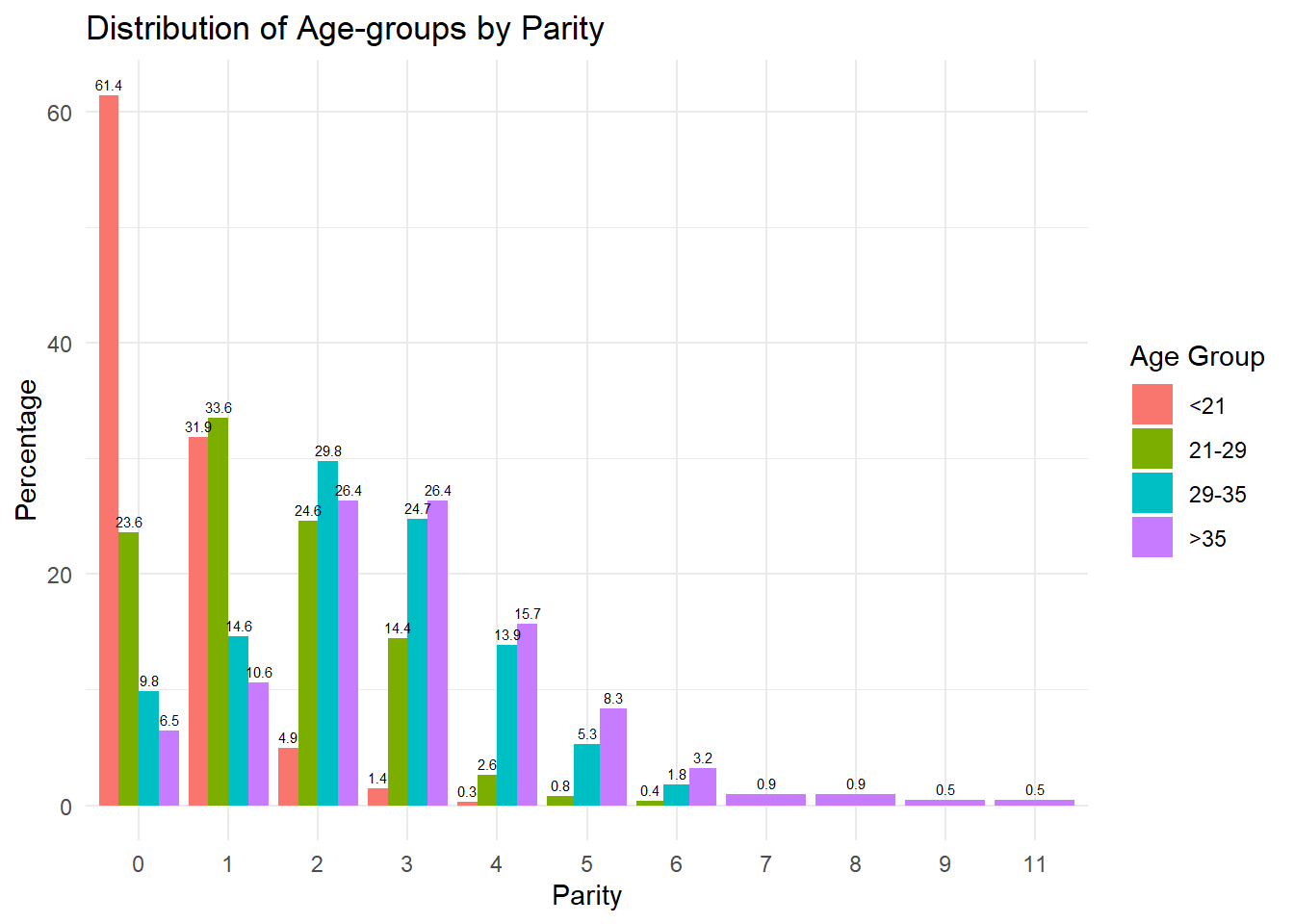
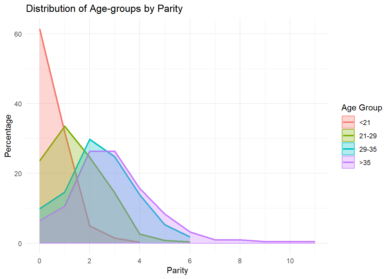
The distribution patterns suggest a trend where younger women (<21) predominantly have their first child, and as age increases, women are more likely to have higher parity deliveries. The 29-35 and >35 age groups, in particular, show a significant percentage of deliveries at higher parity levels, indicating that some women are indeed delaying childbirth to later ages.
We turn our attention next to non-completed or undelivered pregnancies or pregnancies without delivery, the count-difference between gravidarity and parity.This may reflect the state of family planning.
#### GAP: Pregnancy - Delivery gap
```{r echo=FALSE, warning=FALSE, message=FALSE}
# Load required libraries
library(dplyr)
library(ggplot2)
library(knitr)
# Read data
ob_data_tbl_xtra_initial <- readRDS("All Factored Complete Ready OB Dataset for Analytics.RDS") %>%
dplyr::select(-adm_date, -delivery_date) %>%
mutate(grav_fct = factor(grav),
para_fct = factor(para),
age_group = cut(age, breaks = c(-Inf, 21, 29, 35, Inf), labels = c("<21", "21-29", "29-35", ">35")),
age_group = factor(age_group))
# Special count for pending first deliveries
ob_data_filtered <- ob_data_tbl_xtra_initial %>%
mutate(corrected_para = if_else(baby_sq > 1, para - 1, para),
para.xtr= if_else(corrected_para==0, 1, corrected_para))
#grav.xtr= if_else(corrected_para==0 & grav==1, 1, grav))
# # Correct para based on baby_sq condition
# ob_data_corrected <- ob_data_filtered %>%
# mutate(corrected_para = if_else(baby_sq > 1, para - 1, para))
# Calculate the number of pregnancies without delivery
ob_data_preg_without_delivery <- ob_data_filtered%>%
mutate(preg_without_delivery = grav - para.xtr)
# Summarize the data by age group
summary_data_gap <- ob_data_preg_without_delivery %>%
group_by(age_group) %>%
summarise(total_pregnancies = sum(grav),
total_deliveries = sum(para.xtr),
total_preg_without_delivery = sum(preg_without_delivery),
incidence_rate = (total_preg_without_delivery / total_pregnancies * 100),
annual_incidence_rate = round(incidence_rate/9*4,0))
# Display the summary table
kable(summary_data_gap, caption = "Incidence of Pregnancies without Delivery by Age Group")
# Test for statistical significance:
# Assuming the dataframe is named summary_data_gap and has the required columns
# Creating the contingency table
contingency_table <- as.table(rbind(summary_data_gap$total_deliveries, summary_data_gap$total_preg_without_delivery))
colnames(contingency_table) <- summary_data_gap$age_group
rownames(contingency_table) <- c("total_deliveries", "total_preg_without_delivery")
# Performing the chi-square test
chi_square_test <- chisq.test(contingency_table)
# Displaying the results
p_val <- round(chi_square_test$p.value, 4)
cat("p_value =", p_val, "\n")
# Plot the incidence rates by age group
ggplot(summary_data_gap, aes(x = age_group, y = annual_incidence_rate, fill = age_group)) +
geom_bar(stat = "identity") +
labs(title = "Incidence of Pregnancies without Delivery by Age Group",
x = "Age Group",
y = "Incidence Rate (%)",
fill = "Age Group") +
theme_minimal()
overall_gap_annual <- round((sum(summary_data_gap$total_preg_without_delivery)/sum(summary_data_gap$total_pregnancies))*100/9*4,0)
##By Zip:
# Summarize the data by ZIP & age group
gap_zip.df <- ob_data_preg_without_delivery %>%
group_by(zip, age_group) %>%
summarise(total_pregnancies = sum(grav),
total_deliveries = sum(para.xtr),
total_preg_without_delivery = sum(preg_without_delivery),
incidence_rate = (total_preg_without_delivery / total_pregnancies * 100),
annual_incidence_rate = round(incidence_rate/9*4,0)) %>%
select(zip, age_group, total_preg_without_delivery) %>%
pivot_wider(names_from = age_group, values_from = total_preg_without_delivery)
# Calculate column sums
col_sums <- colSums(gap_zip.df[,-1], na.rm = TRUE)
# Apply the percentage calculation
gap_zip.df.prcnt <- gap_zip.df %>%
mutate(across(`<21`:`>35`, ~ round(. / col_sums[as.character(cur_column())] * 100, 1))) %>%
mutate(across(`<21`:`>35`, ~ replace_na(., 0)))
kableExtra::kable(gap_zip.df.prcnt, caption ="Pregnancies without Delivery, by ZIP code")
# Step 2: Sum observed counts for each age group
observed_counts <- colSums(gap_zip.df.prcnt[,-1], na.rm = TRUE)
# Step 3: Calculate expected counts assuming uniform distribution
total_count <- sum(observed_counts)
num_age_groups <- length(observed_counts)
expected_counts <- rep(total_count / num_age_groups, num_age_groups)
# Step 4: Perform chi-squared test
chisq_test <- chisq.test(observed_counts, p = expected_counts / total_count)
# Extract the p-value
p_value <- chisq_test$p.value
# View the p-value
cat("p_value =", p_value, "\n")
```
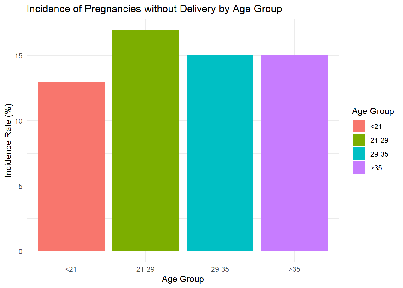
For our patient population, annually, an average of **```r overall_gap_annual```%** of pregnancies were not delivered. There is a statistically significant association between age group and pregnancy outcome (p = ```r p_val```). This suggests that the likelihood of pregnancies resulting in delivery or not, differs significantly across the different age groups.
When considering the annual incidence rate:
- Age group 21-29 has the highest annual incidence rate of pregnancies without delivery (17 per year).
- Age group <21 has the lowest annual incidence rate (13 per year).
- Age groups 29-35 and >35 have similar annual incidence rates (15 per year).
These findings suggest that women in the 21-29 age group experience the highest rate of pregnancies without delivery, while the youngest group (<21) has the lowest rate. The older age groups (29-35 and >35) have intermediate rates. This could imply that younger women (<21) and older women (>35) have different risk factors or behaviors affecting pregnancy outcomes compared to women in their late 20s.
_Of note: there is no significant variation by zip code._
Overall, the significant association and the annual incidence rates highlight important age-related differences in pregnancy outcomes, which could be crucial for targeted interventions and healthcare planning.
Numbers were derived by adding the gravidarity and subtracting parity, while crediting one imminent delivery to P0; and accounting for multiple gestation.
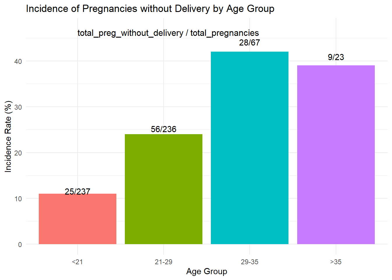
For only the first-ever delivery alone (Para 0), here is the outcome:
```{r echo=FALSE, warning=FALSE, message=FALSE}
# Load required libraries
library(dplyr)
library(ggplot2)
library(knitr)
# Read data
ob_data_tbl_xtra_initial <- readRDS("All Factored Complete Ready OB Dataset for Analytics.RDS") %>%
dplyr::select(-adm_date, -delivery_date) %>%
mutate(grav_fct = factor(grav),
para_fct = factor(para),
age_group = cut(age, breaks = c(-Inf, 21, 29, 35, Inf), labels = c("<21", "21-29", "29-35", ">35")),
age_group = factor(age_group))
# Include only current pending first deliveries only, so para == 0
ob_data_filtered <- ob_data_tbl_xtra_initial %>%
filter(para == 0)
# Calculate the number of pregnancies without delivery
ob_data_preg_without_delivery <- ob_data_filtered %>%
mutate(preg_without_delivery = grav - para)
# Summarize the data by age group
summary_data <- ob_data_preg_without_delivery %>%
group_by(age_group) %>%
summarise(total_pregnancies = sum(grav),
total_deliveries = n(),
total_preg_without_delivery = sum(grav) - total_deliveries,
incidence_rate = round(total_preg_without_delivery / total_pregnancies * 100, 0))
# Display the summary table
kable(summary_data, caption = "Incidence of Pregnancies without Delivery **for primips** by Age Group")
# Plot the incidence rates by age group
ggplot(summary_data, aes(x = age_group, y = incidence_rate, fill = age_group)) +
geom_bar(stat = "identity") +
geom_text(aes(label = paste0(total_preg_without_delivery, "/", total_pregnancies)),
position = position_stack(vjust = 1.05)) +
labs(title = "Incidence of Pregnancies without Delivery by Age Group",
x = "Age Group",
y = "Incidence Rate (%)",
fill = "Age Group") +
annotate("text", x = 1, y = max(summary_data$incidence_rate) + 5,
label = "total_preg_without_delivery / total_pregnancies",
hjust = 0, vjust = 1, size = 4, color = "black") +
theme_minimal() +
theme(legend.position = "none")
overall_incidence_rate <- round(sum(summary_data$total_preg_without_delivery)/sum(summary_data$total_pregnancies)*100,0)
##by ZIP code
library(dplyr)
library(tidyr)
# Step 1: Summarize the data
summarized_df <- ob_data_preg_without_delivery %>%
group_by(zip, age_group) %>%
summarise(total_pregnancies = sum(grav),
total_deliveries = n(),
total_preg_without_delivery = sum(grav) - total_deliveries,
incidence_rate = round(total_preg_without_delivery / total_pregnancies * 100, 0)) %>%
select(zip, age_group, total_preg_without_delivery) %>%
pivot_wider(names_from = age_group, values_from = total_preg_without_delivery)
# View the summarized data
#print(summarized_df)
# Step 2: Calculate column sums
col_sums <- colSums(summarized_df[,-1], na.rm = TRUE)
# Step 3: Calculate percentages
percent_df <- summarized_df %>%
mutate(across(`<21`:`>35`, ~ round(. / col_sums[as.character(cur_column())] * 100, 1))) %>%
mutate(across(`<21`:`>35`, ~ replace_na(., 0)))
# View the data with percentages
#print(percent_df)
kableExtra::kable(percent_df, caption = "Pregnancies without Delivery at time of First Delivery, by ZIP code")
##plotting top 4 zipcodes:
# Manually extracted data
data <- tibble::tribble(
~zip, ~`<21`, ~`21-29`, ~`29-35`, ~`>35`,
"93901", 0, 1.8, 0.0, 0.0,
"93905", 48, 32.1, 35.7, 11.1,
"93906", 4, 21.4, 21.4, 0.0,
"93907", 4, 7.1, 0.0, 0.0,
"93925", 0, 0.0, 0.0, 0.0,
"93926", 0, 0.0, 0.0, 0.0,
"93927", 32, 16.1, 14.3, 77.8,
"93930", 4, 3.6, 25.0, 11.1,
"93933", 0, 0.0, 0.0, 0.0,
"93955", 0, 0.0, 0.0, 0.0,
"93960", 8, 16.1, 0.0, 0.0,
"95012", 0, 1.8, 3.6, 0.0,
"95039", 0, 0.0, 0.0, 0.0,
"99999", 0, 0.0, 0.0, 0.0
)
# Transform the data into long format
long_data <- data %>%
pivot_longer(cols = `<21`:`>35`, names_to = "age_group", values_to = "percentage")
# Filter the data to retain only the specified zip codes
filtered_data <- long_data %>%
filter(zip %in% c("93905", "93906", "93927", "93930"))
# Ensure the age groups are in the correct order
filtered_data$age_group <- factor(filtered_data$age_group, levels = c("<21", "21-29", "29-35", ">35"))
# Create the area plot with lines
ggplot(filtered_data, aes(x = age_group, y = percentage, fill = zip, group = zip)) +
geom_area(position = "identity", alpha = 0.5) +
geom_line(aes(color = zip), size = 1) +
scale_color_brewer(palette = "Set3") +
scale_fill_brewer(palette = "Set3") +
labs(title = "Percentage of Total Pregnancies Without Delivery at the first delivery by Age Group and Top Four Zip Codes",
x = "Age Group",
y = "Percentage",
fill = "Zip Code",
color = "Zip Code") +
theme_minimal() +
theme(axis.text.x = element_text(angle = 0, hjust = 0.5))
#facet
ggplot(filtered_data, aes(x = age_group, y = percentage, fill = zip, group = zip)) +
geom_area(position = "identity", alpha = 0.5) +
geom_line(aes(color = zip), size = 1) +
scale_color_brewer(palette = "Set3") +
scale_fill_brewer(palette = "Set3") +
labs(title = "Percentage of Total Pregnancies Without Delivery at the first delivery by Age Group and Top Four Zip Codes",
x = "Age Group",
y = "Percentage",
fill = "Zip Code",
color = "Zip Code") +
theme_minimal() +
theme(axis.text.x = element_text(angle = 0, hjust = 0.5)) +
facet_wrap(~zip, ncol = 2)
# Step 4: Sum observed counts for each age group
observed_counts <- colSums(summarized_df[,-1], na.rm = TRUE)
# Step 5: Calculate expected counts assuming uniform distribution
total_count <- sum(observed_counts)
num_age_groups <- length(observed_counts)
expected_counts <- rep(total_count / num_age_groups, num_age_groups)
# View observed and expected counts
# print(observed_counts)
# print(expected_counts)
# Step 6: Perform chi-squared test
chisq_test <- chisq.test(observed_counts, p = expected_counts / total_count)
# Extract the p-value
p_value <- chisq_test$p.value
# View the p-value
#print(p_value)
cat("p_value =", p_value, "\n")
```
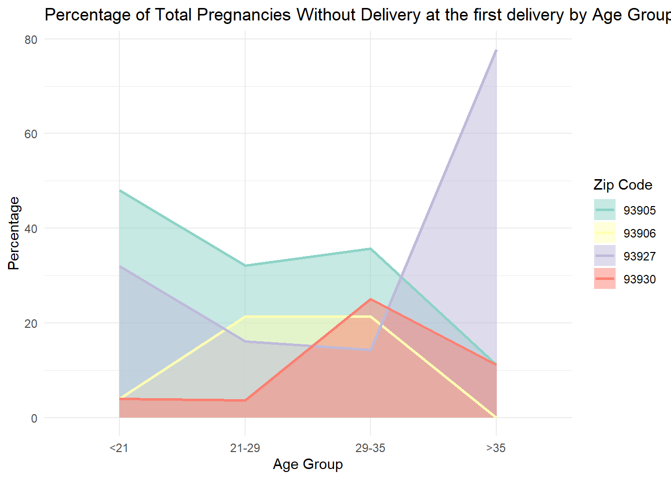
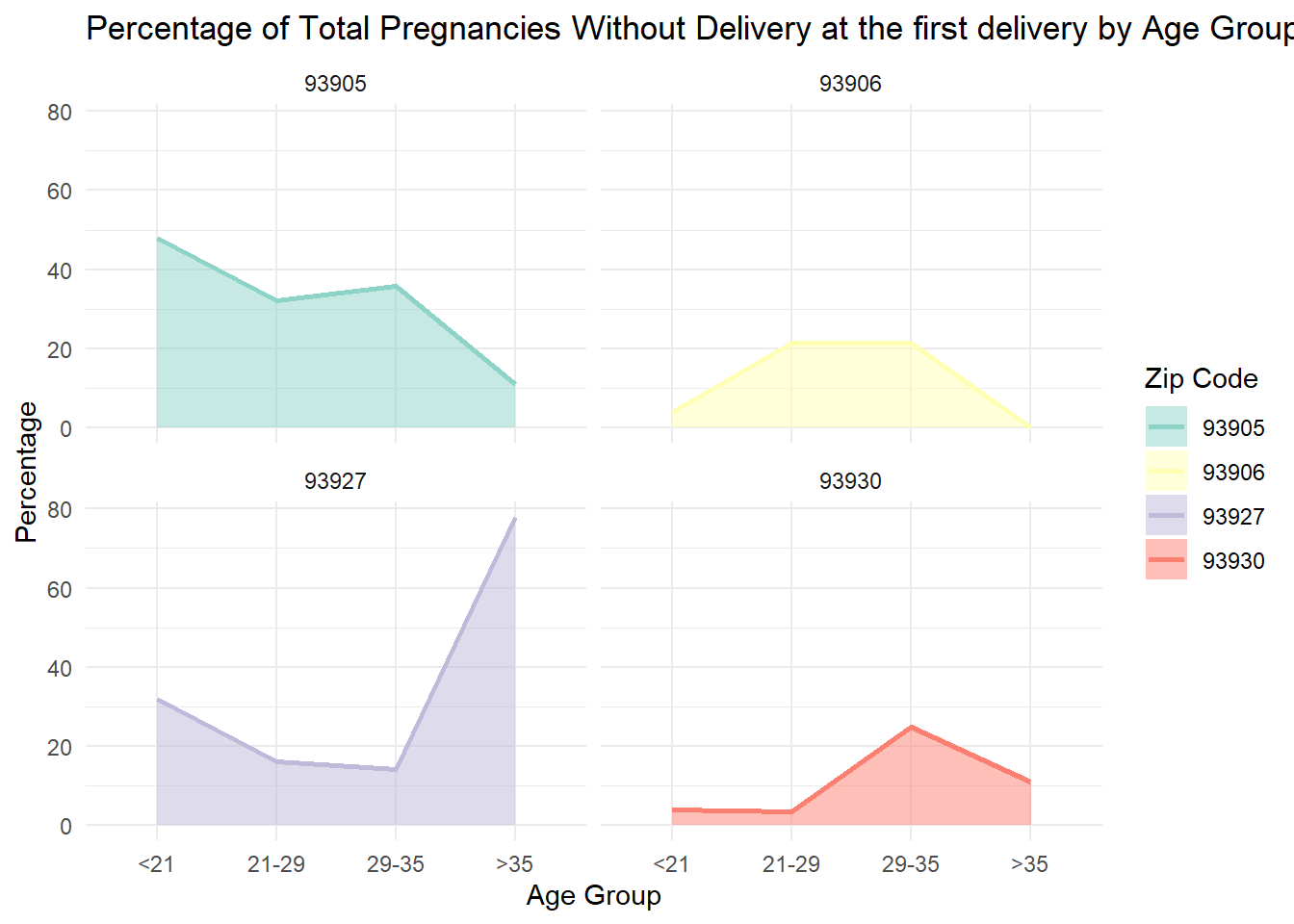
Focusing on first deliveries only, for every 4 delivered pregnancies, one pregnancy was not delivered, given an overall not-delivered incidence rate of **```r overall_incidence_rate```%**. At the time of the first deliveries __only__, there is a significant variance by zip code:
- 93905 has highest delivery gaps in age-group <21, least in >35; even in the rest of the groups
- 93906 has least gap in <21 and >35; rest are even
- 93927 has the highest gap in >35 followed by <21; rest are even
- 93930 has the least gap in 21-29 and <21, highest gap in 29-35, followed by >35
Thus, regarding pregnancies without delivery disparity _at the time of the first delivery_, the data may show a pattern (See plot above) of:
- high disparity at younger ages and low disparity for older ages in 93905;
- high disparity for the middle age groups and low disparity for the younger and the older ages in 93906;
- high disparity for the younger and the older age groups and low disparity for the middle age groups for 93927;
- high disparity for the older age groups and low disparity for the younger age groups for 93930
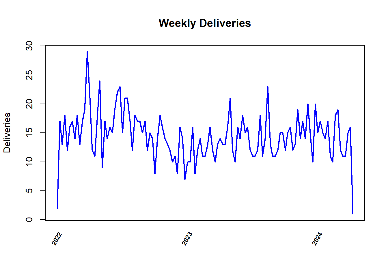
Our records were collected on a continuum of time, so let's take a look. The time series plot is based on weekly deliveries: One can guesstimate the average weekly delivery and well as get a hint as to the trending of weekly deliveries.
### Time Series
```{r echo=FALSE, warning=FALSE, message=FALSE}
library(dplyr)
library(lubridate)
library(plotly)
# Example data transformation
tst <- ob_data_chr %>%
mutate(delivery_date = as.Date(delivery_date),
week_start = floor_date(delivery_date, "week")) %>%
group_by(week_start) %>%
summarise(deliveries = sum(event, na.rm = TRUE)) %>%
ungroup()
deliveries_ts <- ts(tst$deliveries, start = c(2022, 1), frequency = 52)
# Plot the time series with basic customizations
# Customize the x-axis
dates <- seq.Date(from = as.Date("2022-01-01"), by = "week", length.out = length(tst$deliveries))
# Extract year and week number
years <- format(dates, "%Y")
weeks <- as.numeric(format(dates, "%V")) # ISO week numbers from 1-52
# Correct the week number for the last week if it exceeds 52
weeks[weeks > 52] <- 52
# Combine year and week number with conditional year display
formatted_dates <- ifelse(weeks == 1, years, weeks)
# Create x-axis labels at year boundaries and weekly
year_changes <- which(weeks == 1)
week_indices <- seq(1, length(dates), by = 1)
library(ggplot2)
library(plotly)
dates <- seq.Date(from = as.Date("2022-01-01"), by = "week", length.out = length(tst$deliveries))
data <- data.frame(Date = dates, Deliveries = tst$deliveries)
# Create the ggplot with updated linewidth aesthetic
p <- ggplot2::ggplot(data, aes(x = Date, y = Deliveries)) +
geom_line(color = "blue", linewidth = .5) + # Use `linewidth` instead of `size`
scale_x_date(date_labels = "%Y", date_breaks = "1 year") +
labs(title = "Weekly Deliveries", y = "Deliveries", x = "") +
theme_minimal() +
theme(axis.text.x = element_text(angle = 60, hjust = 1, vjust = 1))
# Print the ggplot to verify it
#p
# Convert ggplot to plotly
plotly::ggplotly(p)
```
### Data
Delivery Data for our patients at NMC is kept in NMC OB Delivered Log repository; it captures the following types and categories of information relevant to our analysis:
#### DATA FIELDS
```{r echo=FALSE, warning=FALSE, message=FALSE}
library(knitr)
col_names_nmc <- names(ob_data_chr)
# Omit the last 9 column names
col_names_nmc <- head(col_names_nmc, -12)
# Determine the number of rows needed for three columns
n <- length(col_names_nmc)
n_rows <- ceiling(n / 3)
# Pad the column names with NA to fit the matrix
col_names_nmc <- c(col_names_nmc, rep(NA, 3 * n_rows - n))
# Create a matrix with 3 columns
col_matrix <- matrix(col_names_nmc, ncol = 3, byrow = TRUE)
# Convert the matrix to a data frame for better printing
col_df <- as.data.frame(col_matrix)
# Print the table using kable for better formatting in Quarto
kableExtra::kable(col_df, col.names = NULL, caption = "Data Field Names")
```
To facilitate analyses, we initially added these derived columns below:
```{r echo=FALSE, warning=FALSE, message=FALSE}
column_names <- data.frame(Column_Names = names(ob_data_chr))
derived_cols <- data.frame(column_names[(nrow(column_names) - 12):nrow(column_names), ])
colnames(derived_cols) =NULL
derived_cols_df <- data.frame(Derived_column = derived_cols,
Explanation = c("gestational age in DAYS", "Admission-to-Delivery time", "grav minus para", "Delivery", "Duration: Delivery time minus Admit time",
"Duration ranges", "Age ranges used by UDS", "High Risk OB by definition", "Consolidated intrapartum conditions",
"Consolidated labor types", "Consolidated presentation","Consolidated Delivery method" , "PreTerm / Non-Preterm, informed by Clustering"))
kable(derived_cols_df, caption = "Derived Fields")
```
## Descriptive statistics
```{r echo=FALSE, warning=FALSE, message=FALSE}
# Load necessary libraries
#library(shiny)
library(tableone)
library(dplyr)
library(DT)
library(kableExtra)
ob_data_tbl1 <- readRDS("All Factored Complete Ready OB Dataset for Analytics.RDS") %>%
dplyr::select(-adm_date, -delivery_date) %>%
mutate(cluster = as.factor(cluster))
practiceTbl <- CreateTableOne(data = ob_data_tbl1)
vars <- setdiff(names(ob_data_chr), "gest_age")
practiceTbl_no_gest_age <- CreateTableOne(data = ob_data_tbl1, vars = vars)
#Num vars
num_var_ds <- ob_data_tbl1 %>%
dplyr::select_if(is.numeric) %>%
dplyr::select(-event)
num_var_Tbl <- CreateTableOne(data = num_var_ds)
num_var_prn <- kableone(num_var_Tbl)
# Cat vars
non_num_var_ds <- ob_data_tbl1 %>%
dplyr::select(-c(age, grav, para, weight, apg1, apg5, diff_grav_para, gest_age_days, adm_to_del_tm))
vars <- setdiff(names(non_num_var_ds), "gest_age")
non_num_var_no_gest_age <- CreateTableOne(data = non_num_var_ds, vars = vars)
cat_var_prn <- kableone(non_num_var_no_gest_age)
#print(practiceTbl, showAllLevels = TRUE)
# practiceTbl$CatTable
# practiceTbl$ContTable
#practiceTbl$MetaData
strata_tbl_clst <- CreateTableOne(data = ob_data_tbl1, strata = "cluster", vars = "zip")
#strt_clst_prn <- print(strata_tbl_clst, nonnormal = "cluster", cramVars = "cluster")
strata_tbl_hghRsk <- CreateTableOne(data = ob_data_tbl1, strata = "hghRsk", vars = "zip")
#strt_hghRsk_prn <- print(strata_tbl_hghRsk, nonnormal = "cluster", cramVars = "hghRsk" )
# Use Kable / KableExtra/ kableone
cat_tbl <- kableone(practiceTbl$CatTable)
#kableExtra::kable(cat_tbl, format = "html" )
#cat_tbl
cont_tbl <- kableone(practiceTbl$ContTable)
#kableExtra::kable(cont_tbl, format = "html")
#cont_tbl
strata_tbl_clst <- CreateTableOne(data = ob_data_tbl1, strata = "cluster", vars = "zip")
#print(strata_tbl_clst, nonnormal = "cluster", cramVars = "cluster" )
#kableone(print(strata_tbl_clst, nonnormal = "cluster", cramVars = "cluster" ))
#kableExtra::kable(kableone(strta_zip_clst_prn), format = "html")
strata_tbl_hghRsk <- CreateTableOne(data = ob_data_tbl1, strata = "hghRsk", vars = "zip")
#print(strata_tbl_hghRsk, nonnormal = "cluster", cramVars = "hghRsk" )
#kableone(print(strata_tbl_hghRsk, nonnormal = "cluster", cramVars = "hghRsk"))
#kableExtra::kable(kableone(strta_zip_hghRsk_prn), format = "html")
strata_tbl_clst_rsk <- CreateTableOne(data = ob_data_tbl1, strata = "hghRsk", vars = "cluster")
#print(strata_tbl_hghRsk, nonnormal = "cluster", cramVars = "hghRsk" )
#kableone(print(strata_tbl_clst_rsk, nonnormal = "hghRs", cramVars = "ghgRsk"))
#kableExtra::kable(kableone(strta_zip_hghRsk_prn), format = "html")
```
Let's summarize the CSVS data from NMC Delivery Log, starting with continuous or numerical variables:
### Numeric Variables
```{r echo=FALSE, message=FALSE, warning=FALSE}
num_var_prn
```
Next, we study the delivery frequency among different variables
<!-- ### Frequency View -->
<!-- ```{r echo=FALSE, warning=FALSE, message=FALSE, eval=FALSE} -->
<!-- # Load necessary libraries -->
<!-- #library(shiny) -->
<!-- library(tableone) -->
<!-- library(dplyr) -->
<!-- # Load your data frame -->
<!-- ob_data_tbl1_shny <- readRDS("All Factored Complete Ready OB Dataset for Analytics.RDS") %>% -->
<!-- dplyr::select(-c(age, grav, para, weight, apg1, apg5, diff_grav_para, gest_age_days, adm_to_del_tm, gest_age, adm_date, delivery_date, event, time, baby_sq)) %>% -->
<!-- dplyr::mutate(cluster = as.factor(if_else(cluster == 2, 1, 0))) -->
<!-- ``` -->
Exploratory Data analyses yields rich information. However, we need to proceed with analytics so we can query the data in order to get desired information. We need to know how variables of interest affect one another, and how they compare with one another in their contribution to the results or outcome of interest to us. The outcome of interest to us in OB can be found in prenatal care (before delivery), during delivery; the event of delivery itself and right after delivery.
A pre-delivery outcome, for example, is pre-term (prematurity) status; another is High Risk OB status. During delivery, we are concerned about outcomes categorized by "intrapartal conditions" such as preeclampsia and also "intrapartal events" which encompass abnormal labor dynamics. We want to know: Did delivery occur at all? How long was the time from admission to delivery? What are the chances that at a given time delivery will have occurred, and what percent of patients will have delivered by a certain time? For each of these outcomes or combinations thereof, our interest is how and if variables like maternal age, zip code, parity, high risk status, affected the end-result.
We all are curious to know if and how residential geography affects OB outcomes. We will use zipcode information (the variable, "zip") and a standard MAP to explore this curiosity. High Risk OB is a technical definition; we can explore what contributes to it, as well as determine how it affects other outcomes as mentioned above. A fundamental method in statistical data analytics is to "throw in" all the data, together, "stir it up" and see if the data will settle out in a natural separation into groups--called clustering--that achieves statistical significance. If we can find significant clusters, we can also use them, along with zip and high risk status as probes with which to analyze outcomes.
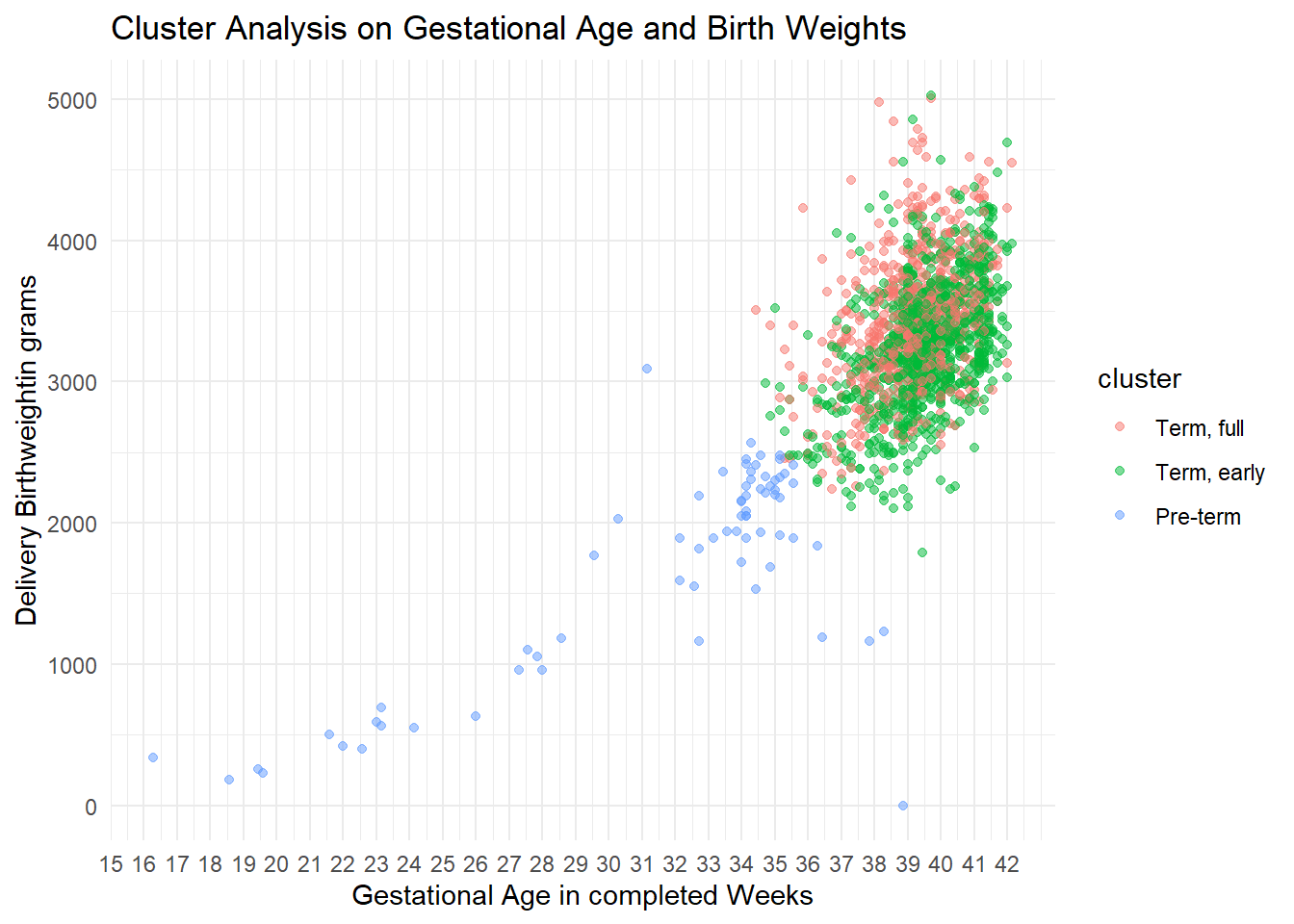
We applied cluster statistics on the data using fetal weight against gestational age: here is our finding:
### Cluster Analysis
Right now, we are going to look into the important OB metrics of Gestational Age and Birth weight of our patients using Cluster Analysis[^1], a useful method in medical research for identifying patterns among patients that help to characterize clinical states and associated risks and treatment outcomes without predefined categories.
[^1]: Cluster analysis is a statistical technique used to group sets of objects in such a way that objects in the same group are more similar to each other than to those in other groups. It is especially useful in medical research for identifying patterns among patients, aiding in understanding behaviors, disease progression, and treatment outcomes without predefined categories.
Using k-means clustering algorithm with a choice of 3 clusters (arbitrary), we obtained these stats and plots:
```{r echo=FALSE, warning=FALSE, message=FALSE}
#Cluster Analysis----
#setwd(getwd())
ob_clustering <- ob_data_fctr %>%
dplyr::select(age, gest_age_days, weight)
ob_clustering_scaled <- scale(ob_clustering)
# Cluster Analysis
set.seed(333)
# Perform K-means clustering
k <- 3
kmeans_result <- kmeans(ob_clustering_scaled, centers = k, nstart = 25)
# Add the cluster assignments to the original dataset
#Remove current var cluster
ob_data_fctr$cluster <- NULL
ob_data_fctr$cluster <- as.factor(kmeans_result$cluster)
# Map numeric cluster IDs to meaningful names
cluster_names <- c("Term, full", "Term, early", "Pre-term")
names(cluster_names) <- 1:3
ob_data_fctr$cluster <- factor(ob_data_fctr$cluster, levels = 1:3, labels = cluster_names)
# Now, summarizing clusters with across
cluster_summary <- ob_data_fctr %>%
group_by(cluster) %>%
summarise(
across(
.cols = c(gest_age_days, weight),
.fns = ~ round(mean(.), 0),
.names = "mean {.col}"
),
count = n(),
percent = round((n() / nrow(ob_data_fctr)) * 100, 1)
)
#kable(cluster_summary, caption = "Cluster Stats")
# Plotting
library(ggplot2)
p <- ggplot2::ggplot(ob_data_fctr, aes(x = gest_age_days, y = weight, color = cluster)) +
geom_point(alpha = 0.5) +
#geom_hline(yintercept = 3000, linetype = "dashed", color = "red") +
#geom_vline(xintercept = 259, linetype = "dashed", color = "blue") +
theme_minimal() +
scale_x_continuous(
name = "Gestational Age in completed Weeks", # Rename the x-axis to "Weeks"
breaks = seq(0, max(ob_data_fctr$gest_age_days), by = 7), # Set breaks every 7 days
labels = function(x) floor(x / 7) # Convert days to floor weeks
) +
labs(title = "Cluster Analysis on Gestational Age and Birth Weights",
x = "Gestational Age", y = "Delivery Birthweightin grams")
p
```
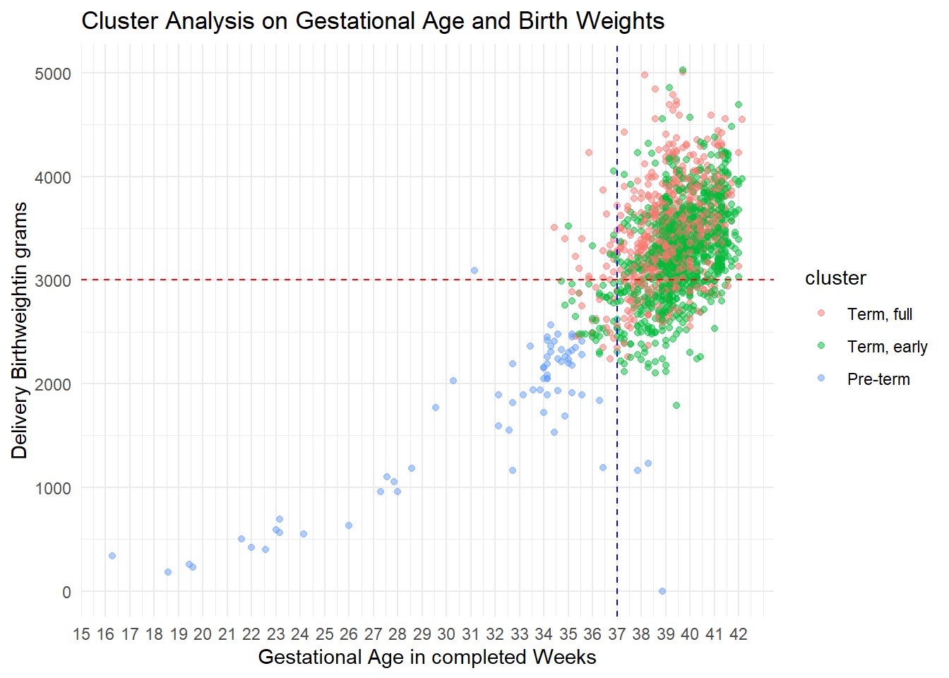
Can we identify this cluster grouping using known and relevant OB metrics for birth weight and gestational age categorization? Yes:
```{r echo=FALSE, warning=FALSE, message=FALSE}
# Plotting
library(ggplot2)
id_clust <- p +
geom_hline(yintercept = 3000, linetype = "dashed", color = "red") +
geom_vline(xintercept = 259, linetype = "dashed", color = "blue")
id_clust
```
```{r echo=FALSE, warning=FALSE, message=FALSE}
clst_smm <- cluster_summary %>%
data.frame()
#kable(cluster_summary, caption = "Cluster Stats")
kableExtra::kable(clst_smm, caption = "Cluster Stats", format = "html", table.attr = "class='table' style='font-size: 14px; width: auto !important;'") %>%
kableExtra::kable_styling(bootstrap_options = "striped", full_width = FALSE, position = "center", font_size = 14)
```
The plot shows the separation of a left lower quad (LLQ) cluster from an un-separated 2 other clusters. Further analysis shows that the LLQ cluster is statistically significantly different from either of the 2 other clusters, while this is not the case between these 2 clusters themselves. By adding the 3000 GRAM birth weight dashed horizontal line and the 37 week dashed vertical line, representing the demarcations for SGA and Preterm respectively we find a correspondence between SGA and preterm delivery, a widely known outcome. The clusters were named after this finding, as: Pre-term; Term, early; and Term, full (latter two are from 37 weeks and over). CAVEAT: Actual preterm deliveries as defined by gestational age (alone) under 37 weeks account for only **`r prcnt_preterm`%** of the deliveries, compared to the cluster group here defined by both SGA AND Preterm (**`r clst_smm[3,5]`%**); both are relatively small numbers compared to the total number of deliveries.
## High Risk OB
Let's officially define "High Risk OB", based on maternal age greater than 35, diagnosis of HTN or Preeclampsia, DM and (for CSVS) multiple gestation and or non-vertex presentation. By these criteria, **`r prcnt_hghRsk`%** are classified as High Risk.
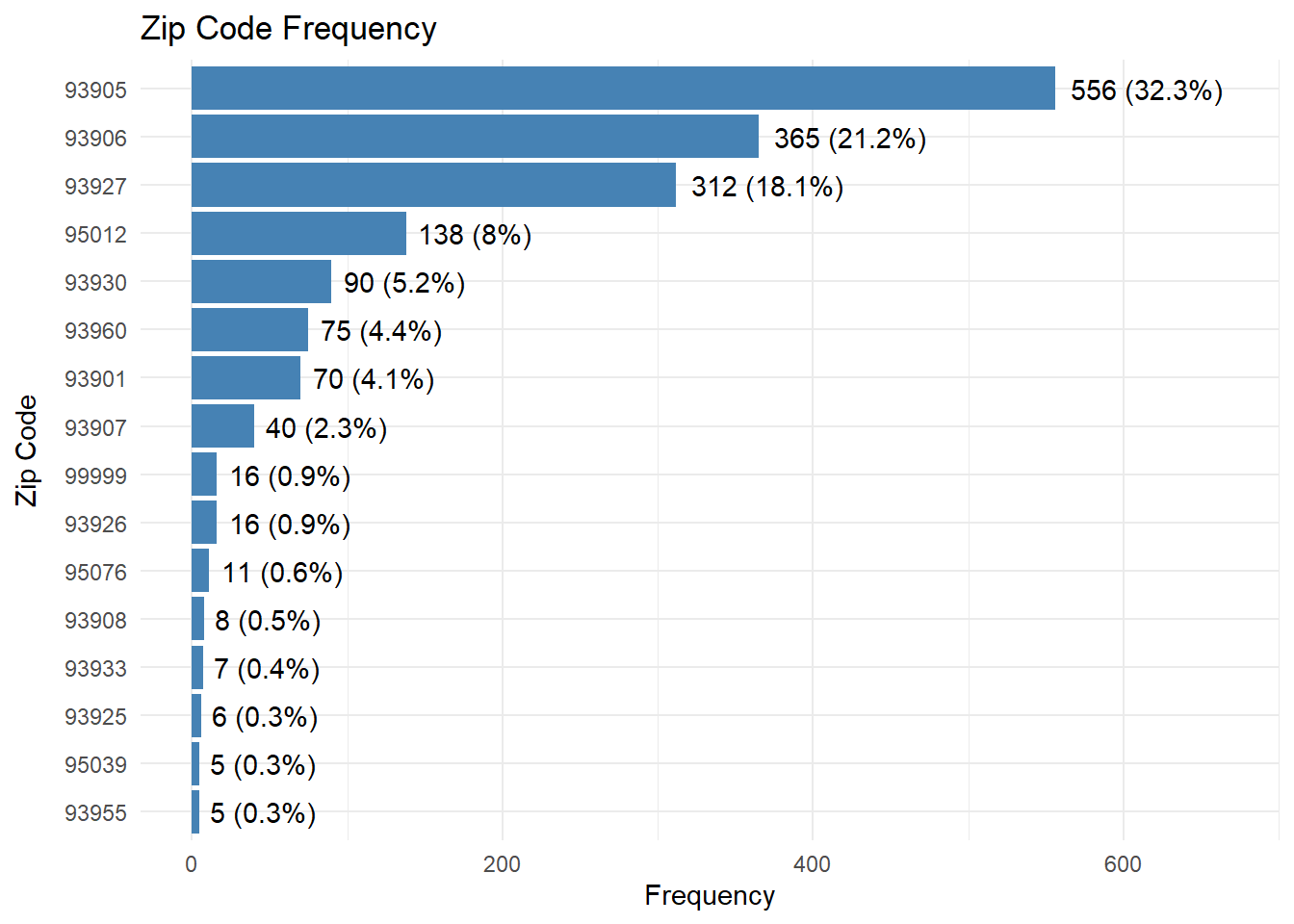
## Service Area by Zipcode
Moving on to zip codes...what is CSVS OB service area? Let's now turn our attention to where our patients come from using a zipcode information (--99999 represents no zip code entered);
```{r echo=FALSE, warning=FALSE, message=FALSE}
library(tableone)
library(dplyr)
library(knitr)
library(kableExtra)
library(tidyr)
library(tibble)
ob_data_tbl2 <- readRDS("All Factored Complete Ready OB Dataset for Analytics.RDS") %>%
dplyr::select(-adm_date, -delivery_date) %>%
mutate(cluster = as.factor(cluster))
# Create the table
zip <- CreateTableOne(data = ob_data_tbl2, vars = "zip")
# Convert to a clean data frame
zip_df <- as.data.frame(print(zip, printToggle = FALSE))
# Print the table to HTML
kableExtra::kable(zip_df, format = "html", caption = "Deliveries by Zip Code", table.attr = "class='table' style='font-size: 14px; width: auto !important;'") %>%
kableExtra::kable_styling(bootstrap_options = "striped", full_width = FALSE, position = "center", font_size = 14)
# ggplot horizontal bar plot
zip_df_plt <- zip_df %>%
rownames_to_column(var = "zip") %>%
slice(-1:-2) %>% # Remove the first two rows
separate(Overall, into = c("freq", "percent"), sep = "\\(") %>%
mutate(freq = as.numeric(trimws(freq)),
percent = as.numeric(gsub("[()%]", "", percent)))
# Print the resulting data frame
#print(zip_df_plt)
library(ggplot2)
# Create the bar plot
p <- ggplot2::ggplot(zip_df_plt, aes(x = reorder(zip, freq), y = freq)) +
geom_bar(stat = "identity", fill = "steelblue") +
geom_text(aes(label = paste0(freq, " (", round(freq / sum(freq) * 100, 1), "%)")), hjust = -0.1) +
coord_flip() +
labs(title = "Zip Code Frequency",
x = "Zip Code",
y = "Frequency") +
theme_minimal() +
expand_limits(y = max(zip_df_plt$freq) * 1.2) # Adjust y-axis limit to provide space for labels
# Print the plot
print(p)
# Save the plot with adjusted dimensions if needed
ggsave("zip_code_frequency_plot.png", plot = p, width = 10, height = 6)
```
The top 5 are 93905 (one-third of all deliveries), 93906 (one-fifth), 93927 (one-sixth); 95012 (one-twelfth), 93930 (one-twentieth). One thing stands out: considering its size and straddling location, 99308 is a sparse draw for CSVS deliveries.
Let's place this information within the context of a map of the County:
### Map
```{r echo=FALSE, warning=FALSE, message=FALSE}
library(leaflet)
library(sf)
library(dplyr)
library(RColorBrewer)
# Load spatial and data
zip_code_sf <- readRDS("CSVS service area with Zipcode and Population with sf and shp.RDS")
ob_data_map <- readRDS("Working OB Dataset.RDS")
# Summarize data by ZIP code
ob_data_map <- ob_data_map %>%
count(zip)
# Convert ZIP codes to character
ob_data_map$zip <- as.character(ob_data_map$zip)
zip_code_sf$ZCTA5CE20 <- as.character(zip_code_sf$ZCTA5CE20)
# Convert zip_code_sf to WGS84 datum
zip_code_sf <- st_transform(zip_code_sf, crs = 4326)
# Perform the join
ob_data_map_joined <- zip_code_sf %>%
left_join(ob_data_map, by = c("ZCTA5CE20" = "zip"))
# Check for missing values and handle them
ob_data_map_joined$n[is.na(ob_data_map_joined$n)] <- 0
# Create a color palette function
colorPalette <- colorBin(palette = "YlOrRd", domain = ob_data_map_joined$n, bins = 5)
# Generate the leaflet map
ob_data_map <- leaflet(data = ob_data_map_joined) %>%
addTiles() %>%
addPolygons(
fillColor = ~colorPalette(n),
color = "#BDBDC3",
fillOpacity = 0.7,
weight = 1,
opacity = 1,
highlight = highlightOptions(
weight = 3,
color = "#666",
fillOpacity = 0.7,
bringToFront = TRUE
),
label = ~paste("ZIP Code:", ZCTA5CE20, "<br/>Count:", n),
labelOptions = labelOptions(
direction = 'auto',
noHide = FALSE,
textOnly = TRUE
)
) %>%
addLegend(
pal = colorPalette,
values = ~n,
opacity = 0.7,
title = "Count",
position = "bottomright"
) %>%
setView(lng = -121.895, lat = 36.674, zoom = 9)
ob_data_map
```
This map shows that zipcode 93908 sitting smack within "CSVS territory" has extremely low deliveries. Census Information[^2] reveals that this discrepancy is demographical (socioeconomic) and related to CSVS usual drawing pool. This zipcode, 93908 ("Salinas - Corral De Tierra"), compared with say, 93905:
[^2]: (source: <https://www.unitedstateszipcodes.org/93908/>, viewed 2024-05-27)
- has primarily white residents Vs "primarily other race" residents
- has Median Household Income \$108,093 Vs \$41,607
- has Median Home Value \$616,000, Vs \$203,400[^3]
[^3]: (source: <https://www.unitedstateszipcodes.org/93908/>, viewed 2024-05-27)
# Data Analysis
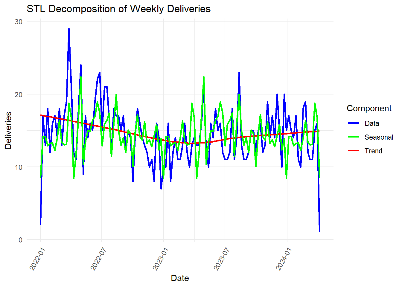
Having identified certain parameters of interest (Zip code distribution, Prematurity and High Risk), let's proceed to see what our data is telling us. We will start by taking another look at the weekly deliveries, to check for patterns (seasonality) and overall direction of the total number of deliveries (trend); and then, predict number of deliveries as forecast for the next quarter.
Is there seasonality to the deliveries? Do we have a trend?
##### Time series decomposition
```{r, echo=FALSE, message=FALSE, warning=FALSE}
library(dplyr)
library(lubridate)
library(forecast)
library(ggplot2)
library(tidyr)
# Example data transformation
tst <- ob_data_chr %>%
mutate(delivery_date = as.Date(delivery_date),
week_start = floor_date(delivery_date, "week")) %>%
group_by(week_start) %>%
summarise(deliveries = sum(event, na.rm = TRUE)) %>%
ungroup()
# Create the time series object
deliveries_ts <- ts(tst$deliveries, start = c(2022, 1), frequency = 52)
#Original ts:
plot(deliveries_ts, xaxt = "n", main = "Weekly Deliveries", ylab = "Deliveries", xlab = "", col = "blue", lwd = 2)
# Rotate x-axis labels 60 degrees
par(xpd = TRUE)
# text(x = seq(2022, 2022 + (length(tst$deliveries) - 1) / 52, by = 1 / 52),
# y = par("usr")[3] - 1,
# labels = formatted_dates,
# srt = 60,
# adj = 1,
# cex = 0.7)
# Add year labels
text(x = seq(2022, 2022 + (length(tst$deliveries) - 1) / 52, by = 1 / 52)[year_changes],
y = par("usr")[3] - 2,
labels = years[year_changes],
srt = 60,
adj = 1,
cex = 0.7, font = 2)
# STL decomposition facet:
stl_fit <- stl(deliveries_ts, s.window = 20)
# Extract the components
components <- as.data.frame(stl_fit$time.series)
components$date <- seq.Date(from = as.Date("2022-01-01"), by = "week", length.out = nrow(components))
components$data <- tst$deliveries
# Reorder the components for plotting
components_long <- components %>%
dplyr::select(date, data, seasonal, trend) %>%
pivot_longer(cols = -date, names_to = "component", values_to = "value")
# Plot the components ordered by Data, Seasonal, Trend
plotly::ggplotly(
ggplot2::ggplot(components_long, aes(x = date, y = value, color = component)) +
geom_line(size = 1) +
facet_wrap(~component, scales = "free_y", ncol = 1) +
labs(title = "STL Decomposition of Weekly Deliveries",
y = "Value",
x = "Date",
color = "Component") +
scale_color_manual(values = c("data" = "blue", "seasonal" = "green", "trend" = "red")) +
theme_minimal() +
theme(axis.text.x = element_text(angle = 60, hjust = 1))
)
###
#STL decomposition superimposition
# Perform STL decomposition
stl_fit <- stl(deliveries_ts, s.window = "periodic")
# Extract the components
components <- as.data.frame(stl_fit$time.series)
components$date <- seq.Date(from = as.Date("2022-01-01"), by = "week", length.out = nrow(components))
components$data <- tst$deliveries
# Adjust the seasonal component to match the scale of the data
components$seasonal_adjusted <- components$seasonal + mean(components$data)
# Superimpose data, trend, and adjusted seasonal components
ggplot2::ggplot(components, aes(x = date)) +
geom_line(aes(y = data, color = "Data"), size = 1) +
geom_line(aes(y = trend, color = "Trend"), size = 1) +
geom_line(aes(y = seasonal_adjusted, color = "Seasonal"), size = 1) +
labs(title = "STL Decomposition of Weekly Deliveries",
y = "Deliveries",
x = "Date",
color = "Component") +
scale_color_manual(values = c("Data" = "blue", "Trend" = "red", "Seasonal" = "green")) +
theme_minimal() +
theme(axis.text.x = element_text(angle = 60, hjust = 1))
```
The top graph shows the same weekly deliveries time series seen earlier. The second and third panels tease out the series to extract seasonality information and trend, respectively. The last panel superimposes the seasonality and trend graphs on the original time series. We can see a trend that "trough-ed" around end of the first quarter of 2023 and is rising since then. The seasonality graph nearly matches the original data, indicating that there is a significant seasonal variation in weekly deliveries among our patients.
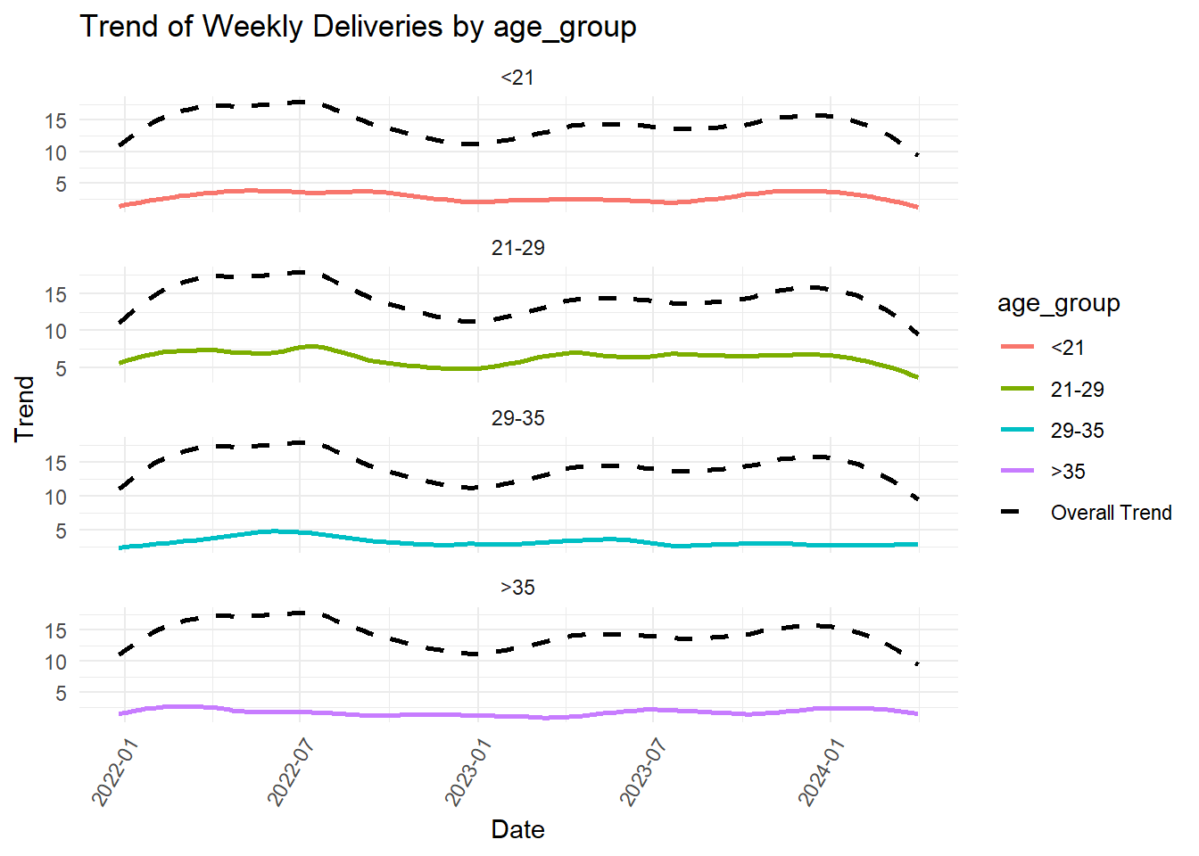
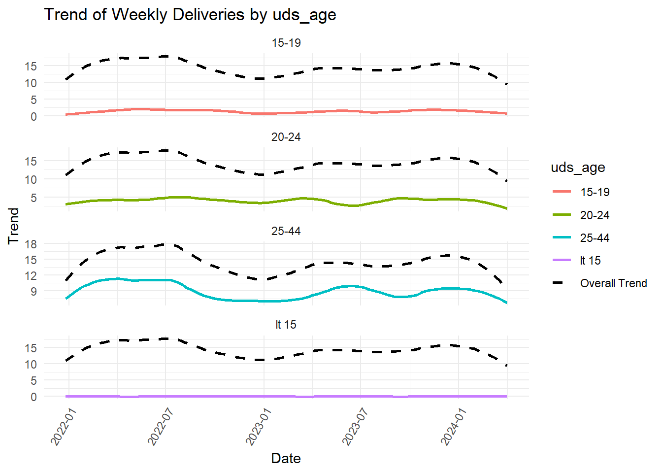
What might account for the trough? Below we compare the original (full data) trend with the trend of each of the components of various variables to look for patterns.
#### Checking for trend disparity
```{r echo=FALSE, warning=FALSE, message=FALSE}
library(dplyr)
library(lubridate)
library(ggplot2)
library(tidyr)
library(scales)
library(trend)
# Load your dataset
ob_data_fctr <- readRDS("All Factored Complete Ready OB Dataset for Analytics.RDS")
# Ensure date is in the correct format
ob_data_fctr_1 <- ob_data_fctr %>%
mutate(delivery_date = as.Date(delivery_date))
# Get top 5 zip codes by delivery frequency
top_zips <- ob_data_fctr_1 %>%
count(zip, sort = TRUE) %>%
top_n(5, n) %>%
pull(zip)
# Refactor the zip column to include only the top 5 zip codes
ob_data_fctr_2 <- ob_data_fctr_1 %>%
mutate(zip = factor(zip, levels = top_zips))
# Cut age into specified groups
ob_data_fctr_3 <- ob_data_fctr_2 %>%
mutate(age_group = cut(age, breaks = c(-Inf, 21, 29, 35, Inf), labels = c("<21", "21-29", "29-35", ">35")))
# Compute the overall trend
overall_trend <- ob_data_fctr_3 %>%
mutate(week_start = floor_date(delivery_date, "week")) %>%
group_by(week_start) %>%
summarise(deliveries = sum(event, na.rm = TRUE), .groups = 'drop') %>%
mutate(trend = predict(loess(deliveries ~ as.numeric(week_start), span = 0.3)))
# Function to create trend plot for a given variable
create_trend_plot <- function(data, var) {
if (var == "zip") {
# Filter only top 5 zip codes
data <- data %>% filter(zip %in% top_zips)
}
# Aggregate weekly deliveries for the given variable
ts_data <- data %>%
mutate(week_start = floor_date(delivery_date, "week")) %>%
group_by(week_start, !!sym(var)) %>%
summarise(deliveries = sum(event, na.rm = TRUE), .groups = 'drop') %>%
ungroup() %>%
complete(week_start, !!sym(var), fill = list(deliveries = 0))
# Apply Loess smoothing to capture the trend
ts_data <- ts_data %>%
group_by(!!sym(var)) %>%
mutate(trend = predict(loess(deliveries ~ as.numeric(week_start), span = 0.3))) %>%
ungroup()
# Plot the trend
ggplot2::ggplot(ts_data, aes(x = week_start, y = trend, color = !!sym(var))) +
geom_line(size = 1) +
facet_wrap(as.formula(paste("~", var)), scales = "free_y", ncol = 1) +
geom_line(data = overall_trend, aes(x = week_start, y = trend, color = "Overall Trend"), linetype = "dashed", size = 1, inherit.aes = FALSE) +
scale_color_manual(values = c(setNames(hue_pal()(length(unique(ts_data[[var]]))), unique(ts_data[[var]])), "Overall Trend" = "black")) +
labs(title = paste("Trend of Weekly Deliveries by", var),
y = "Trend",
x = "Date",
color = var) +
theme_minimal() +
theme(axis.text.x = element_text(angle = 60, hjust = 1))
}
# Function to calculate Mann-Kendall trend test p-values
calculate_trend_tests <- function(data, var) {
data %>%
mutate(week_start = floor_date(delivery_date, "week")) %>%
group_by(week_start, !!sym(var)) %>%
summarise(deliveries = sum(event, na.rm = TRUE), .groups = 'drop') %>%
filter(!is.na(!!sym(var))) %>%
group_by(!!sym(var)) %>%
summarise(
mann_kendall_p = mk.test(deliveries)$p.value
) %>%
mutate(variable = var)
}
# List of variables to test
variables <- c("zip", "hghRsk", "cluster", "age_group", "uds_age")
# Calculate trend tests for each variable and combine results
trend_results_list <- lapply(variables, function(var) {
calculate_trend_tests(ob_data_fctr_3, var)
})
# Combine all results into one data frame
trend_results <- bind_rows(trend_results_list)
# Concatenate the variable levels with the variable name and remove NA columns
# Convert variables to characters before using coalesce
trend_results <- trend_results %>%
mutate(
zip = as.character(zip),
hghRsk = as.character(hghRsk),
cluster = as.character(cluster),
age_group = as.character(age_group),
uds_age = as.character(uds_age),
variable_level = paste(variable, coalesce(zip, hghRsk, cluster, age_group, uds_age), sep = ": ")
) %>%
select(variable_level, mann_kendall_p)
# Add interpretative column
trend_results <- trend_results %>%
mutate(interpretation = ifelse(mann_kendall_p <= 0.05, "Significant trend, contributes uniquely", "No significant trend, does not contribute uniquely"))
# Print the cleaned p-values summary table with interpretation
#print(trend_results)
#kableExtra::kable(trend_results, caption = "Trends Contribution Effect")
# Create and print trend plots for each specified variable
zip_plot <- create_trend_plot(ob_data_fctr_3, "zip")
print(zip_plot)
hghrsk_plot <- create_trend_plot(ob_data_fctr_3, "hghRsk")
print(hghrsk_plot)
ob_data_fctr_3$cluster <- as.factor(ob_data_fctr_3$cluster)
cluster_plot <- create_trend_plot(ob_data_fctr_3, "cluster")
print(cluster_plot)
age_plot <- create_trend_plot(ob_data_fctr_3, "age_group")
print(age_plot)
uds_age_plot <- create_trend_plot(ob_data_fctr_3, "uds_age")
print(uds_age_plot)
kableExtra::kable(trend_results, caption = "Trends Contribution Effect")
```
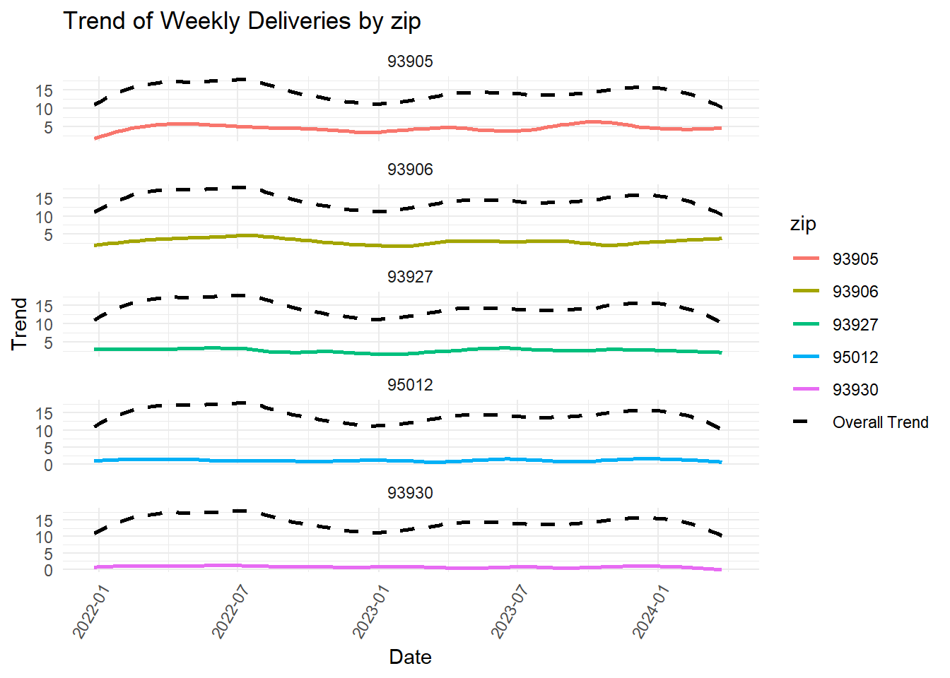
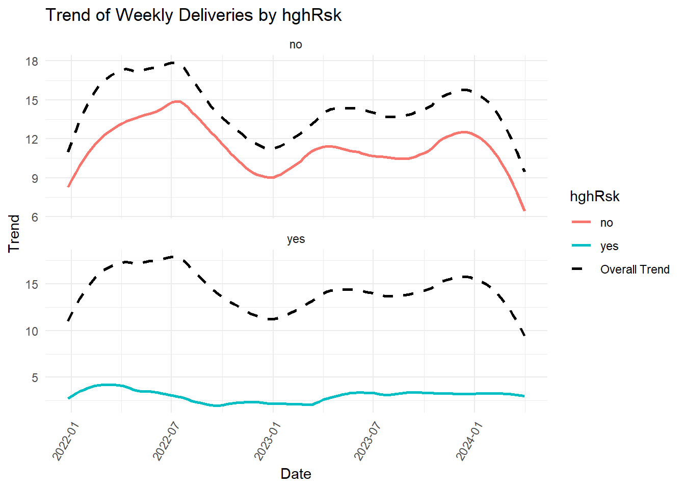
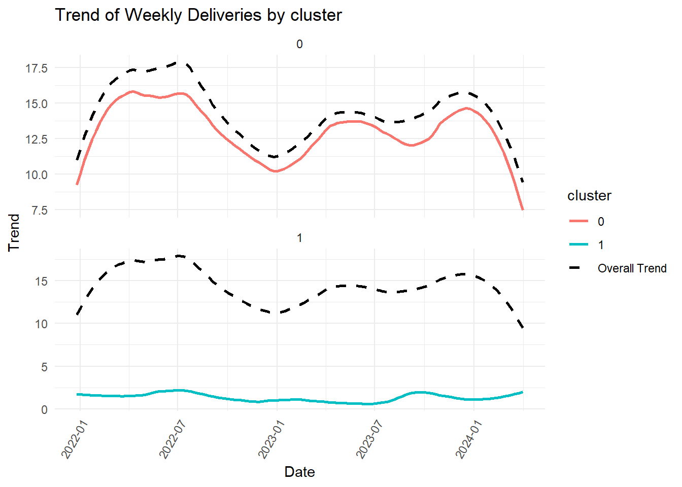
If the trend of the original data ("Overall Trend) parallels the variable's trend visually, the latter must be contributing significantly to the shape and direction of the former. However, we must rely on p-values for statistical significance. Thus, the following contribute significantly to the trend that we observed:
- zip: 93930
- hghRsk: no
- age_group: 29-35
but, not the rest of the zipcodes, cluster, age groups (including UDS age group)
An important and practical goal of data analysis is to make future forecasts. Based on the weekly delivery numbers for 117 weeks or nine quarters, we can predict the following quarter's performance: check the plot, and then the table for comparison between actual and predicted data. (Use the cursor cross-mark to expand any segment by pressing the button and dragging the mouse)
### Time Series Forecasts
```{r echo=FALSE, warning=FALSE, message=FALSE}
# Load necessary libraries
library(dplyr)
library(ggplot2)
library(lubridate)
library(timetk)
library(tsibble)
library(prophet)
library(Metrics)
library(feasts)
library(fabletools)
library(plotly)
# Summarize deliveries by week
ob_data_ts <- readRDS("Working OB Dataset.RDS") %>%
mutate(delivery_date = as.Date(delivery_date),
week_start = floor_date(delivery_date, "week")) %>%
group_by(week_start) %>%
summarise(deliveries = sum(event, na.rm = TRUE)) %>%
ungroup()
# Ensure date columns are Date objects
ob_data_ts$week_start <- as.Date(ob_data_ts$week_start)
# Prepare data for prophet
prophet_data <- ob_data_ts %>%
rename(ds = week_start, y = deliveries)
# Fit prophet model with weekly seasonality
prophet_model <- prophet(prophet_data, weekly.seasonality = TRUE)
# Generate future dataframe
future <- make_future_dataframe(prophet_model, periods = 13, freq = "week")
# Forecast
forecast <- predict(prophet_model, future)
# Ensure forecast dataframe ds column is Date object
forecast$ds <- as.Date(forecast$ds)
# Combine historical data and forecast
combined_data <- bind_rows(
prophet_data %>% mutate(type = "Historical"),
forecast %>% mutate(type = "Forecast", y = yhat) %>% dplyr::select(ds, y, type)
)
# Check for and remove duplicate rows if any
combined_data <- combined_data %>%
distinct(ds, .keep_all = TRUE)
# Round forecast values
forecast <- forecast %>%
mutate(yhat = round(yhat))
# Extract forecast values as DataFrame
forecast_df <- combined_data %>%
filter(type == "Forecast") %>%
dplyr::select(ds, y) %>%
rename(Date = ds, Forecast = y)
# Plot: Full historical + forecast with explicit weeks for x-axis
p_ts_frcst <- ggplot2::ggplot() +
geom_line(data = combined_data, aes(x = ds, y = y, color = type), size = 1) +
scale_x_date(date_breaks = "1 week", date_labels = "%Y-%U") +
labs(title = "Forecast for the Next Quarter",
x = "Week",
y = "Number of Deliveries",
color = "Legend") +
scale_color_manual(values = c("Historical" = "black", "Forecast" = "orange")) +
theme_minimal() +
theme(
plot.title = element_text(hjust = 0.5, size = 14, face = "bold"),
axis.title = element_text(size = 12),
axis.text = element_text(size = 10),
legend.title = element_text(size = 12),
legend.text = element_text(size = 10),
axis.text.x = element_text(angle = 45, hjust = 1)
)
#print(p_ts_frcst)
ggplotly(p_ts_frcst)
# Output forecast values as DataFrame
forecast_df <- forecast_df %>% mutate(Forecast = round(Forecast)) %>% data.frame(.)
kableExtra::kable(forecast_df, caption = "Next Quarter's Weekly Deliveries Forecast")
```
We are going to continue the analysis of our data using zip-code distribution, Clustering and High Risk OB before moving to generalized analyses.
How does zip code affect the distribution of outcomes like Preterm (derived from cluster analysis)and High Risk OB? We will throw in another interesting outcome, Delivery Method (vaginal versus Caeserian section)?
### Zip Code effect
```{r echo=FALSE, warning=FALSE, message=FALSE}
library(dplyr)
library(tableone)
ob_data_tbl3 <- readRDS("All Factored Complete Ready OB Dataset for Analytics.RDS") %>%
mutate(cluster = as.factor(cluster)) %>%
dplyr::select(-adm_date, -delivery_date)
strata_tbl_clst_zip <- CreateTableOne(data = ob_data_tbl3, strata = "cluster", vars = "zip")
#print(strata_tbl_clst, nonnormal = "cluster", cramVars = "cluster" )
kableone(strata_tbl_clst_zip, nonnormal = "cluster", cramVars = "cluster" , caption = "Distribution of Preterm by Zip code")
#kableExtra::kable(kableone(strta_zip_clst_prn), format = "html")
strata_tbl_hghRsk_zip <- CreateTableOne(data = ob_data_tbl3, strata = "hghRsk", vars = "zip")
#print(strata_tbl_hghRsk, nonnormal = "cluster", cramVars = "hghRsk" )
kableone(strata_tbl_hghRsk_zip, cramVars = "hghRsk", caption = "Distribution of High Risk OB by Zip code")
#kableExtra::kable(kableone(strta_zip_hghRsk_prn), format = "html")
strata_tbl_del_zip <- CreateTableOne(data = ob_data_tbl3, strata = "del_method_cnsldt", vars = "zip")
#print(strata_tbl_hghRsk, nonnormal = "cluster", cramVars = "hghRsk" )
kableone(strata_tbl_del_zip, cramVars = "del_method_cnsldt", caption = "Distribution of Delivery Methods by Zip code")
#kableExtra::kable(kableone(strta_zip_hghRsk_prn), format = "html")
```
First, always check the p-values for the various distribution tables.
The answer is: there is no significant difference in the relative distribution, among and within different zip codes, of Pre-term deliveries (p=0.508), High Risk OB (p=0.792), Delivery Method (p=0.976).
What about the High Risk OB and the outcomes of Preterm & Delivery Method?
```{r echo=FALSE, warning=FALSE, message=FALSE}
strata_tbl_clst_rsk <- CreateTableOne(data = ob_data_tbl3, strata = "cluster", vars = "hghRsk")
#print(strata_tbl_hghRsk, nonnormal = "cluster", cramVars = "hghRsk" )
kableone(strata_tbl_clst_rsk, nonnormal = "cluster", cramVars = "hghRsk", caption = "Distribution of Preterm by High Risk OB")
#kableExtra::kable(kableone(strta_zip_hghRsk_prn), format = "html")
strata_tbl_del_rsk <- CreateTableOne(data = ob_data_tbl3, strata = "del_method_cnsldt", vars = "hghRsk")
#print(strata_tbl_hghRsk, nonnormal = "cluster", cramVars = "hghRsk" )
kableone(strata_tbl_del_rsk, nonnormal = "del_method_cnsldt", cramVars = "hghRsk", caption = "Distribution of Delivery Method by High Risk OB")
#kableExtra::kable(kableone(strta_zip_hghRsk_prn), format = "html")
```
With a p-value \<0.001, a statistically significant difference is obvious in the distribution of Cesarean sections compared to Vaginal deliveries among High Risk OB. The same holds true for Preterm distribution: a significantly higher percent are in High Risk group than non-Preterm (39.8% Vs 19.2%, p-value \<0.001).
Finally, same question for Preterm and outcomes of High Risk and Delivery Method:
```{r echo=FALSE, warning=FALSE, message=FALSE}
strata_tbl_rsk_clst <- CreateTableOne(data = ob_data_tbl3, strata = "hghRsk", vars = "cluster")
#print(strata_tbl_hghRsk, nonnormal = "cluster", cramVars = "hghRsk" )
kableone(strata_tbl_rsk_clst, nonnormal = "cluster", cramVars = "hghRsk", caption = "Distribution of Preterm by High Risk OB")
#kableExtra::kable(kableone(strta_zip_hghRsk_prn), format = "html")
strata_tbl_del_clst <- CreateTableOne(data = ob_data_tbl3, strata = "del_method_cnsldt", vars = "cluster")
#print(strata_tbl_hghRsk, nonnormal = "cluster", cramVars = "hghRsk" )
kableone(strata_tbl_del_clst, nonnormal = "cluster", cramVars = "del_method_cnsldt", caption = "Distribution of Preterm by Delivery Method")
#kableExtra::kable(kableone(strta_zip_hghRsk_prn), format = "html")
```
- The distribution of High Risk OB is significantly higher compared with non_High Risk among Preterm deliveries (p=\<0.001).
- The distribution of C-sections is significantly higher compared with vaginal delivery among Preterm deliveries (p=0.039).
<!-- Next, we perform correlation analysis on our data -->
<!-- ### Correlation Analysis (Spearman method) -->
<!-- Correlation -->
<!-- : Correlation is a statistical measure that describes the strength and direction of a relationship between two variables. It ranges from -1 to 1, where values close to 1 or -1 indicate strong positive or negative relationships, respectively, and values close to 0 indicate no relationship. -->
<!-- We have prepared an interactive table to facilitate the exercise. Keep in mind that the included p-value determines whether there is a statistical significance or not. ***There are 15x14 possible pair-combinations, so, think, "parsimony".*** -->
```{r echo=FALSE, warning=FALSE, message=FALSE}
#library(shiny)
library(XICOR)
library(dplyr)
library(ggplot2)
library(DT)
# Assuming the dataset is loaded here
ob_data_clst_xi <- readRDS("All Factored Complete Ready OB Dataset for Analytics.RDS") %>%
mutate(cluster = as.factor(cluster)) %>%
dplyr::select(zip, lbr_type_cnsldt, membrane_rupture, intrapartal_conditions,
presentation_cnsldt, conditions_cnsldt, uds_age, adm_to_del_tm_cat, hghRsk, del_method_cnsldt, cluster,
age, grav, para, diff_grav_para) %>%
mutate(across(c(zip, lbr_type_cnsldt, membrane_rupture, intrapartal_conditions,
presentation_cnsldt, conditions_cnsldt, uds_age, adm_to_del_tm_cat, hghRsk, del_method_cnsldt, cluster), as.factor)) %>%
mutate(across(c(zip, lbr_type_cnsldt, membrane_rupture, intrapartal_conditions,
presentation_cnsldt, conditions_cnsldt, uds_age, adm_to_del_tm_cat, hghRsk, del_method_cnsldt, cluster), as.numeric))
```
# Hospital: Labor & Delivery
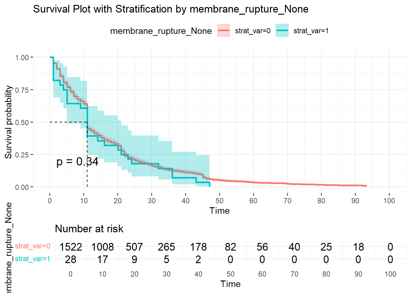
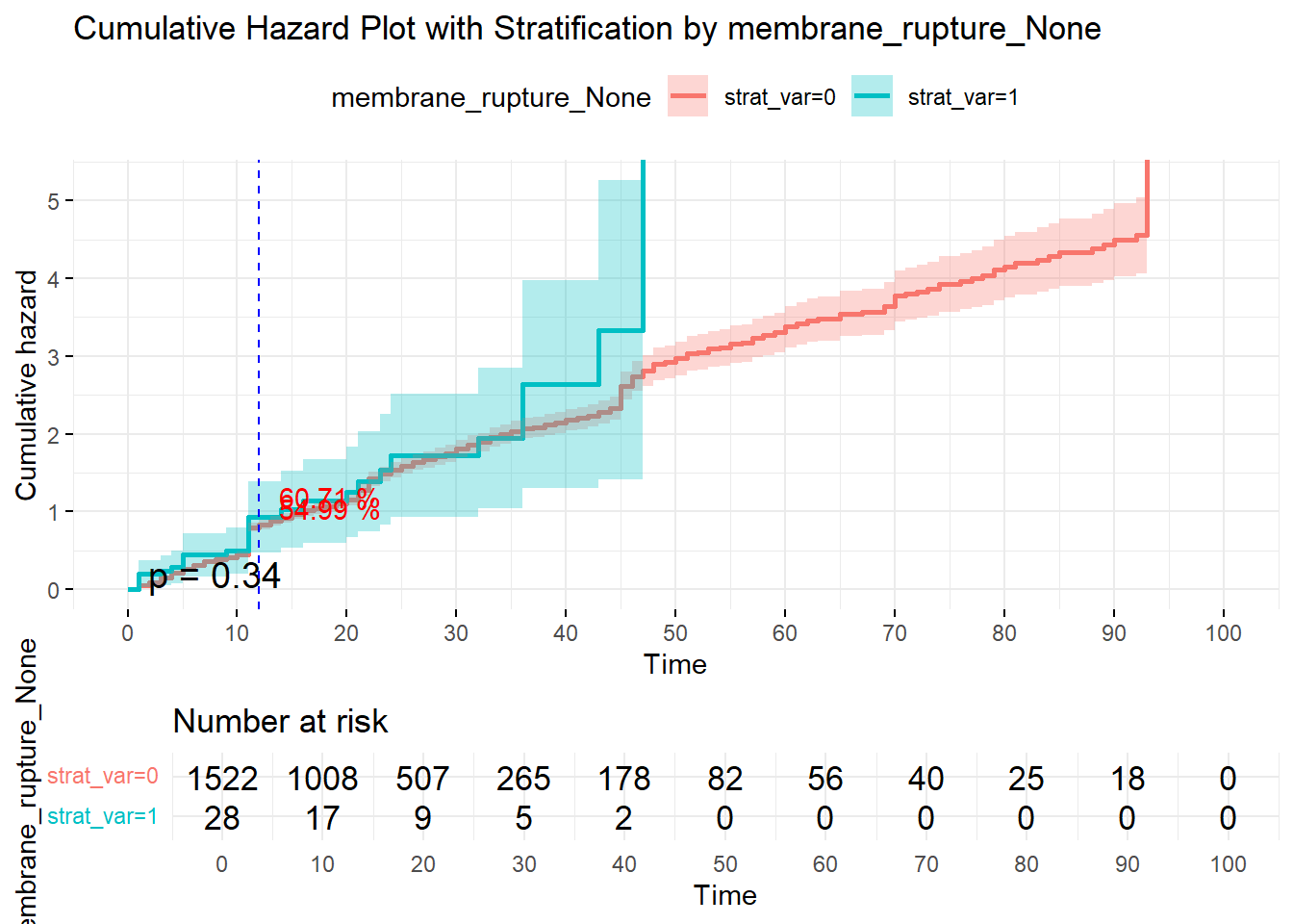
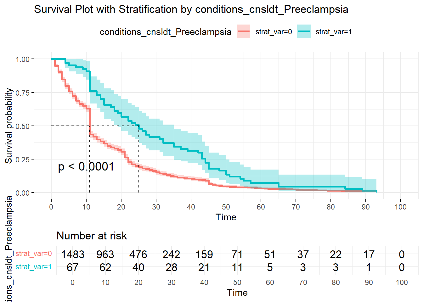
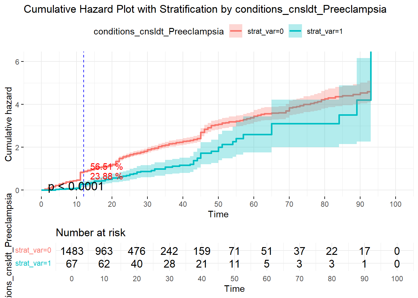
Let's now shift our attention to hospital events related to OB care. First, we will extend the previous analyses to hospital events. Then, we will use a different method of analysis known as Survival Analysis (SA) or by Time-to-Event (TTE) Analysis to probe our data. The hospital **event of interest is Delivery**; along with related matters of labor type, delivery method, intrapartal events and intrapartal conditions. Here are the variables and their respective member-items:
### Variables
```{r echo=FALSE, warning=FALSE, message=FALSE}
# List of factor variable names
library(dplyr)
library(tidyr)
ob_data_tbl4 <- readRDS("All Factored Complete Ready OB Dataset for Analytics.RDS") %>%
dplyr::select(-adm_date, -delivery_date) %>%
mutate(cluster= as.factor(cluster))
# List of factor variable names
factor_vars <- c("lbr_type_cnsldt", "del_method_cnsldt", "conditions_cnsldt", "intrapartal_events") # Replace with your actual factor variable names
# Function to get levels and create a data frame
get_levels_df <- function(var_name) {
levels_df <- data.frame(
Variable = var_name,
Items = levels(ob_data_tbl4[[var_name]]),
stringsAsFactors = FALSE
)
return(levels_df)
}
# Apply the function to each factor variable and combine the results
levels_list <- lapply(factor_vars, get_levels_df)
combined_levels_df <- bind_rows(levels_list)
# Group by Variable and keep only the first instance of Variable name
formatted_df <- combined_levels_df %>%
group_by(Variable) %>%
mutate(Variable = ifelse(row_number() == 1, Variable, "")) %>%
ungroup()
# Print the formatted data frame
#print(formatted_df)
tableone::kableone(formatted_df)
```
We have consolidated some of the items within their respective original variables and named them with "-cnsldt" appendum.
Below are the frequency and the distribution of deliveries by these variables:
```{r echo=FALSE, warning=FALSE, message=FALSE}
library(tableone)
library(dplyr)
library(knitr)
library(kableExtra)
library(tidyr)
library(tibble)
ob_data_tbl5 <- readRDS("All Factored Complete Ready OB Dataset for Analytics.RDS") %>%
dplyr::select(-adm_date, -delivery_date) %>%
mutate(cluster = as.factor(cluster))
vars <- c("lbr_type_cnsldt", "presentation_cnsldt", "intrapartal_events", "conditions_cnsldt", "del_method_cnsldt")
# Create the table
selected_hosp <- tableone::CreateTableOne(data = ob_data_tbl5, vars = vars)
# Convert to a clean data frame
selected_hosp_df <- as.data.frame(print(selected_hosp, printToggle = FALSE))
# Move row names to a column
selected_hosp_df <- rownames_to_column(selected_hosp_df, var = "RowID")
# Identify and clean header and item rows
selected_hosp_df <- selected_hosp_df %>%
mutate(
Variable = ifelse(grepl("^X\\.*", RowID), "", RowID),
Item = ifelse(grepl("^X\\.*", RowID), gsub("^X\\.*", "", RowID), ""),
Value = Overall
) %>%
dplyr::select(Variable, Item, Value) %>%
fill(Variable, .direction = "down")
# Print the table to HTML
kableExtra::kable(selected_hosp_df, format = "html", caption = "Distribution of Deliveries among Hospital Variables", table.attr = "class='table' style='font-size: 12px; width: auto !important;'") %>%
kableExtra::kable_styling(bootstrap_options = "striped", full_width = FALSE, position = "left", font_size = 12)
```
### Distribution analysis
#### By zip
Like we did with previous situations, we ask if hospital events and hospital conditions at delivery show a biased distribution with regards to zip codes.
```{r echo=FALSE, warning=FALSE, message=FALSE}
ob_data_tbl6 <- readRDS("All Factored Complete Ready OB Dataset for Analytics.RDS") %>%
dplyr::select(-adm_date, -delivery_date) %>%
mutate(cluster = as.factor(cluster))
strata_tbl_lbr_zip <- CreateTableOne(data = ob_data_tbl6, strata = "lbr_type_cnsldt", vars = "zip")
kableone(strata_tbl_lbr_zip, cramVars = "lbr_type_cnsldt", caption = "Distribution of Labor Types by Zip code")
strata_tbl_conditions_zip <- CreateTableOne(data = ob_data_tbl6, strata = "conditions_cnsldt", vars = "zip")
kableone(strata_tbl_conditions_zip, cramVars = "conditions_cnsldt", caption = "Distribution of Intrapartal Conditions by Zip code")
strata_tbl_events_zip <- CreateTableOne(data = ob_data_tbl6, strata = "intrapartal_events", vars = "zip")
kableone(strata_tbl_events_zip, cramVars = "intrapartal_events", caption = "Distribution of Intrapartal Events by Zip code")
```
- For labor types (p-value = 0.142) and intrapartal conditions (p-value = 0.151) there is no significant difference in their distribution among and within the zipcodes.
- A different conclusion for Intrapartal events (p_value = 0.02): Focusing on the 3 most frequent intrapartal events, there is a significant difference in precipitous labor (93905, 93927, 93906); Prolonged Labor \>20 hrs (93905, 93906, 93927); and Prolonged 2nd Stg \>2.5 hr (93905, 93906, 93927); 93905 had the most difference in each category.
#### By High Risk OB
```{r echo=FALSE, warning=FALSE, message=FALSE}
ob_data_tbl7 <- readRDS("All Factored Complete Ready OB Dataset for Analytics.RDS") %>%
dplyr::select(-adm_date, -delivery_date) %>%
mutate(cluster = as.factor(cluster))
strata_tbl_lbr_rsk <- CreateTableOne(data = ob_data_tbl7, strata = "lbr_type_cnsldt", vars = "hghRsk")
kableone(strata_tbl_lbr_rsk, cramVars = "hghRsk", caption = "Distribution of Labor Types by High Risk OB")
strata_tbl_conditions_rsk <- CreateTableOne(data = ob_data_tbl7, strata = "conditions_cnsldt", vars = "hghRsk")
kableone(strata_tbl_conditions_rsk, cramVars = "conditions_cnsldt", caption = "Distribution of Intrapartal Conditions by High Risk OB")
strata_tbl_events_rsk <- CreateTableOne(data = ob_data_tbl7, strata = "intrapartal_events", vars = "hghRsk")
kableone(strata_tbl_events_rsk, cramVars = "intrapartal_events", caption = "Distribution of Intrapartal Events by High Risk OB")
```
High Risk OB, on the other hand, showed significant differences in all three parameters:
- Labor Type (p= \<0.001) : 30% induced; 14% spontaneous -- greater association with labor induction;
- Intrapartal conditions (p = \<0.001): None 16.6% versus 100% Preclampsia, 18.1% infection, and 17.6 % Prolonged Rupture of Membrane
- Intrapartal events (p = 0.002): None 21.9% Vs 10.5% for Precipitous labor < 3hrs, 8.1 % for Prolonged 2nd stage \>2.5 hr and 27.8 % for Prolonged labor \> 20 hr
#### By Preterm:
```{r echo=FALSE, warning=FALSE, message=FALSE}
ob_data_tbl8 <- readRDS("All Factored Complete Ready OB Dataset for Analytics.RDS") %>%
mutate(cluster = as.factor(cluster)) %>%
dplyr::select(-adm_date, -delivery_date)
strata_tbl_lbr_clstr <- CreateTableOne(data = ob_data_tbl8, strata = "lbr_type_cnsldt", vars = "cluster")
kableone(strata_tbl_lbr_clstr, cramVars = "cluster", caption = "Distribution of Labor Types by Preterm")
strata_tbl_conditions_clstr <- CreateTableOne(data = ob_data_tbl8, strata = "conditions_cnsldt", vars = "cluster")
kableone(strata_tbl_conditions_clstr, cramVars = "conditions_cnsldt", caption = "Distribution of Intrapartal Conditions by Preterm")
strata_tbl_events_clstr <- tableone::CreateTableOne(data = ob_data_tbl8, strata = "intrapartal_events", vars = "cluster")
kableone(strata_tbl_events_clstr, cramVars = "intrapartal_events", caption = "Distribution of Intrapartal Events by Preterm")
```
The analysis shows that Preterm
- is significantly associated with different frequencies of different Labor types (p=0.009) AND different intrapartal conditions (p= \<0.001)
- but NOT different intrapartal events (p=0.172)
In summary, for this series of frequency and distribution analysis, we can conclude that High Risk OB has significant impact on Intrapartal events and Intrapartal conditions, as well as Labor Type.
There are many other ways to analyze the data with this method. For example, we can address questions like: _does labor induction lead to more C-sections?_
#### Labor type by Delivery method: an example
```{r echo=FALSE, message=FALSE, warning=FALSE}
example_question <- ob_data_tbl1
strata_tbl_del_method_rsk <- CreateTableOne(data = example_question, strata = "del_method_cnsldt", vars = "lbr_type_cnsldt")
kableone(strata_tbl_del_method_rsk, cramVars = "lbr_type_cnsldt", caption = "Distribution of Delivery Method by Labor type")
```
We show a statistically significant effect (p = <0.001): Induced labor is associated with a higher frequency of Primary C-Section when compared to other delivery types (36.4%), but also when Primary C-Section rate is compared to Vaginal Delivery rate for the labor induction group (36.4% Vs 25.1%). That solves out to **Odds Ratio of 1.70** (We will see Odds Ratio again later); meaning that the odds of having Primary C-Section are 1.7 times higher for labor induction group, and it is statistically significant at p-value <0.001)
#### Delivery method by High Risk OB: an example
Another example: _Is Caesarian section more frequent in High Risk OB?_
```{r echo=FALSE, warning=FALSE, message=FALSE}
example_question_2 <- ob_data_tbl1
strata_tbl_del_method_rsk_2 <- CreateTableOne(data = example_question_2, strata = "del_method_cnsldt", vars = "hghRsk")
kableone(strata_tbl_del_method_rsk_2, cramVars = "del_method_cnsldt", caption = "Distribution of Delivery Method by High Risk")
```
Yes, in fact, at a p-value = \<0.001, the percent distribution is: 44.5%, 32.8%, and 15.6% for C/S-- Primary; C/S-- Repeat; and Vaginal delivery respectively when High Risk OB is a present condition.
Moving on to a different analysis schema: Survival Analysis (SA) or by Time-to-Event (TTE) Analysis.
### Survival Analysis (SA)
Survival or Time-to_Event (TTE) Analysis
: Survival analysis, or time-to-event analysis, is a statistical method used to analyze the expected duration until one or more events occur, such as death or failure. It involves the use of survival functions to estimate the probability of surviving past a certain time point. The Kaplan-Meier (KM) estimator is a non-parametric statistic used to estimate the survival function from observed survival times. Cumulative hazard (cumHaz) functions represent the accumulated risk of the event over time. Hazard ratios (HR) compare the hazard or event rates between two groups, indicating the relative likelihood of the event occurring in one group compared to another.
Survival Analysis can answer the questions:
- What is the probability of being undelivered at a given time after admission? (yields Median Survival)
- What percent of all deliveries would have occurred at a given time after admission? (Cumulative Hazard)
- What is the comparative likelihood of delivery having occurred given a certain condition versus absence of such a condition at a certain time (Hazard Ratio, (HR))?
These are important questions for planning, predictions and for information for patient.
##### Definitions
Here's a definition of terms relevant to Survival or Time-to_Event (TTE) Analysis :
**Event**: *Delivery* or the outcome
There is an associated delivery date with time that defines the event occurrence
**Intervention**: *Admission to the NMC*
A date-time is associated with Intervention
**Interval**: *Duration* of time between Intervention and Event.
**Time**: any *slice* of, or *point* , in time (not Duration) within Interval
**Survival**: *"Survived" Event* at any given Time
**Hazard**: *Risk of Event at any point in time* at any given Time
**Cumulative Hazard**: *Accumulated Risk of event up to a given point in time* at any given time
**Hazard Ratio (HR)**: *Relative hazard rates between two groups at any given point in time* at any given Time
In our case, given that the Event is Delivery, **Survival** means "_survived_ delivery", ie., **delivery has NOT occurred** at the specified Time; or, a status of **undelivered**.
These definitions will facilitate the interpretation of our analyses when we use the popular analytic method called Survival Analysis (SA) or Time to Event (TTE) analysis.
For Survival or TTE Analysis, we will use the method of Cox Proportional Hazards; this permits the taking into account together of all the variables that contribute to an outcome (or event) even while focusing on a particular variable of interest. The data subset will exclude deliveries done before patient had a chance for admission-registration, the latter being the time-stamp to start the clock of Intervention. That leaves **```r sa_data```** deliveries, a substantial **```r sa_data_prcnt```%** of all deliveries.
#### COX Survival, K-M, Cumulative Hazard and Hazard Ratio
Standard plot and example:
###### Cox Surv, CumHaz, strata = ALL
####### General: ALL variables, SA, CumHaz
```{r echo=FALSE, warning=FALSE, message=FALSE}
ob_data_coxph <- readRDS("All Factored Complete Ready OB Dataset for Analytics.RDS") %>%
filter(time >= 0) %>%
dplyr::select(-adm_date, -delivery_date, -labor_type, -intrapartal_conditions, -delivery_method,
-baby_sq, -gest_age, -adm_to_del_tm, -adm_to_del_tm_cat, -presentation) %>%
mutate(cluster = as.factor(cluster))
# One-hot encode categorical variables
categorical_vars <- c("zip", "membrane_rupture", "intrapartal_events", "gender", "uds_age", "hghRsk", "conditions_cnsldt", "lbr_type_cnsldt", "presentation_cnsldt",
"del_method_cnsldt", "cluster")
ob_data_encoded <- dummy_cols(ob_data_coxph, select_columns = categorical_vars, remove_first_dummy = TRUE, remove_selected_columns = TRUE)
ob_data_encoded_coxph <- dummy_cols(ob_data_coxph, select_columns = categorical_vars, remove_first_dummy = TRUE, remove_selected_columns = TRUE)
# Ensure no negative or zero survival times
ob_data_encoded_coxph <- ob_data_encoded_coxph %>%
filter(time > 0)
# Sanitize variable names
sanitize_names <- function(names_vector) {
names_vector <- gsub(" ", "_", names_vector)
names_vector <- gsub(",", "", names_vector)
names_vector <- gsub("<", "lt", names_vector)
names_vector <- gsub(">", "gt", names_vector)
names_vector <- gsub("-", "_", names_vector)
names_vector <- gsub("/", "_", names_vector) # Handle slashes
return(names_vector)
}
colnames(ob_data_encoded_coxph) <- sanitize_names(colnames(ob_data_encoded_coxph))
all_vars <- names(ob_data_encoded_coxph)
all_vars <- setdiff(all_vars, c("time", "event"))
saveRDS(ob_data_encoded_coxph, "OB data encoded ALL VARIABLES for CoxPH.RDS")
cox_model_all <- coxph(as.formula(paste("Surv(time, event) ~", paste(all_vars, collapse = " + "))), data = ob_data_encoded_coxph)
#surv_fit <- survfit(Surv(time, event) ~ data = ob_data_encoded_coxph)
surv_fit <- survfit(cox_model_all, data=ob_data_encoded_coxph)
surv_plot <- ggsurvplot(
surv_fit,
data = ob_data_encoded_coxph,
surv.median.line = "hv",
pval = TRUE,
conf.int = TRUE,
xlim = c(0, 100),
risk.table = TRUE,
break.time.by = 10,
ggtheme = theme_minimal(),
title = paste("Cox Survival Plot without Stratification")
#legend.title = "ALL"
)
print(surv_plot)
# CumHaz
cumhaz_plot <- ggsurvplot(
surv_fit,
data = ob_data_encoded_coxph,
risk.table = TRUE,
pval = TRUE,
fun = "cumhaz",
conf.int = TRUE,
xlim = c(0, 100),
break.time.by = 10,
ggtheme = theme_minimal(),
title = paste("Cox Cumulative Hazard Plot without Stratification")
#legend.title = "ALL"
)
# Extract the number of individuals at risk at time zero
at_risk_zero <- surv_fit$n.risk[1]
# Calculate the time point where 50% of individuals are at risk
half_at_risk_time <- min(surv_fit$time[surv_fit$n.risk <= at_risk_zero / 2])
# Add the line for 50% at risk time
cumhaz_plot$plot <- cumhaz_plot$plot +
geom_vline(xintercept = half_at_risk_time, linetype = "dashed", color = "blue") +
annotate("text", x = half_at_risk_time, y = max(surv_fit$cumhaz),
label = paste("50% At Risk at t =", round(half_at_risk_time, 2)),
color = "blue", vjust = -1.5)
# Print the plot
print(cumhaz_plot)
#print(cumhaz_plot)
```
There's the top plot (Survival Plot) which shows the probability of Survival at any time; and the bottom plot (Cumulative Hazard Plot) which shows accumulated events at any time.
In the top / Survival Plot, the intersecting vertical and horizontal lines determine "median survival (time)": the time at which survival probability is 50% (time at which half the population will have survived (or experienced) the event). Time, for our purposes, is measured in hours since hospital admission registration.
Keeping in mind that for our data,
- "Survival" = not delivered (or undelivered);
- "Event" = "Hazard" = Delivered.
- "Risk" = the risk of Delivery.
We can interpret the top graph as:
- median survival is 12 hours; or,
- the time when half of our patients is __expected__ to be still undelivered is 12 hours; or,
- Our patients have a 50% probability of being undelivered at 12 hours after admission.
For the bottom graph, we determine the time when the cumulative deliveries show 50% still need to deliver (or are still to deliver). It works out to be about 12 hours. Note: it's just a coincidence that the median survival time (the time when half of our patients is still undelivered, based on probability) is also 12 hours.
This method is most informative when used to compare of different variable subsets, for example:
###### Cox Surv, CumHaz --stratified examples
```{r echo=FALSE, warning=FALSE, message=FALSE}
library(survival)
library(survminer)
ob_data_encoded <- readRDS("OB data encoded Significant Variables for CoxPH.RDS")
# Create the Surv object
surv_obj <- Surv(time = ob_data_encoded$time, event = ob_data_encoded$event)
# Create the Cox model using significant variables
cox_model_significant <- coxph(Surv(time, event) ~ age + apg1 + apg5 + gest_age_days +
membrane_rupture_None + intrapartal_events_Precip_Labor_lt3_hrs +
intrapartal_events_Prolonged_Labor_gt20_hrs + uds_age_25_44 +
conditions_cnsldt_Placenta_Previa + conditions_cnsldt_Preeclampsia +
conditions_cnsldt_Preeclampsia_Infection + conditions_cnsldt_Prolonged_ROM +
lbr_type_cnsldt_Induced + lbr_type_cnsldt_Not_Applicable +
lbr_type_cnsldt_Spontaneous, data = ob_data_encoded)
# Choose a categorical variable for stratification
strat_var <- "membrane_rupture_None"
# Add the stratification variable to the data frame
ob_data_encoded$strat_var <- ob_data_encoded[[strat_var]]
# Survival plot with stratification
surv_fit <- survfit(Surv(time, event) ~ strat_var, data = ob_data_encoded)
surv_plot <- ggsurvplot(
surv_fit,
data = ob_data_encoded,
surv.median.line = "hv",
risk.table = TRUE,
pval = TRUE,
conf.int = TRUE,
xlim = c(0, 100),
break.time.by = 10,
ggtheme = theme_minimal(),
title = paste("Survival Plot with Stratification by", strat_var),
legend.title = strat_var
)
# Print the survival plot
print(surv_plot)
# Cumulative hazard plot with stratification
cumhaz_plot <- ggsurvplot(
surv_fit,
fun = "cumhaz",
data = ob_data_encoded,
risk.table = TRUE,
pval = TRUE,
conf.int = TRUE,
xlim = c(0, 100),
break.time.by = 10,
ggtheme = theme_minimal(),
title = paste("Cumulative Hazard Plot with Stratification by", strat_var),
legend.title = strat_var
)
# Choose a fixed time point for the vertical line
fixed_time <- 12
# Extract the number of individuals at risk at time zero for each stratum
n_risk_at_zero <- sapply(1:length(surv_fit$strata), function(i) {
surv_fit$n.risk[1 + sum(head(surv_fit$strata, i - 1))]
})
# Extract the number of individuals at risk at the fixed time point for each stratum
n_risk_at_fixed_time <- sapply(1:length(surv_fit$strata), function(i) {
summary(surv_fit, times = fixed_time, extend = TRUE)$n.risk[i]
})
# Calculate the percentage reduction in the number at risk for each stratum
percent_reduction_at_fixed_time <- 100 * (n_risk_at_zero - n_risk_at_fixed_time) / n_risk_at_zero
# Extract cumulative hazard at the fixed time point for each stratum
cumhaz_at_fixed_time <- sapply(1:length(surv_fit$strata), function(i) {
summary(surv_fit, times = fixed_time, extend = TRUE)$cumhaz[i]
})
# Add the vertical line at the fixed time point
cumhaz_plot$plot <- cumhaz_plot$plot +
geom_vline(xintercept = fixed_time, linetype = "dashed", color = "blue")
# Add labels for cumulative hazard percentage at the fixed time point for each stratum
for (i in 1:length(cumhaz_at_fixed_time)) {
cumhaz_plot$plot <- cumhaz_plot$plot +
annotate("text", x = fixed_time, y = cumhaz_at_fixed_time[i] + (i - 1) * 0.1,
label = paste(round(percent_reduction_at_fixed_time[i], 2), "%"),
color = "red", vjust = -0.5, hjust = -0.2)
}
# Print the plot
print(cumhaz_plot)
```
The example above compares the condition of __membrane-rupture__ with __no membrane-rupture__. First thing to check is the p-value. A p-value of 0.34 is \> 0.05, there is therefore no statistically significant difference among this condition-binary with respect to probability of survival (undelivered); or cumulative hazard (total delivered) at any time. Based on the graph, at 11 hours, the probability of being undelivered is 50% for either of them. At 12 hours (your pick of time; it could have been at 20, 30, or 36 hours) the cumulative hazard (accumulated deliveries) is 55% and 61% respectively, which do not meet the test of statistical significance for being different.
On the other hand, below, when comparing the intrapartal condition, __Preeclampsia present or not__, we can see the difference in Survival (undelivered status) and Cumulative deliveries; p-value \<0.0001. 50% undelivered probability is at ~12-hr mark if no Preeclampsia, but doubles to 25 hours when Preeclampsia is present. At the same time , cumulative delivered is 57% with Preeclampsia absent but only 24% if Preeclampsia is present.
```{r echo=FALSE, warning=FALSE, message=FALSE}
library(survival)
library(survminer)
ob_data_encoded <- readRDS("OB data encoded Significant Variables for CoxPH.RDS")
# Create the Surv object
surv_obj <- Surv(time = ob_data_encoded$time, event = ob_data_encoded$event)
# Create the Cox model using significant variables
cox_model_significant <- coxph(Surv(time, event) ~ age + apg1 + apg5 + gest_age_days +
membrane_rupture_None + intrapartal_events_Precip_Labor_lt3_hrs +
intrapartal_events_Prolonged_Labor_gt20_hrs + uds_age_25_44 +
conditions_cnsldt_Placenta_Previa + conditions_cnsldt_Preeclampsia +
conditions_cnsldt_Preeclampsia_Infection + conditions_cnsldt_Prolonged_ROM +
lbr_type_cnsldt_Induced + lbr_type_cnsldt_Not_Applicable +
lbr_type_cnsldt_Spontaneous, data = ob_data_encoded)
# Choose a categorical variable for stratification
strat_var <- "conditions_cnsldt_Preeclampsia"
# Add the stratification variable to the data frame
ob_data_encoded$strat_var <- ob_data_encoded[[strat_var]]
# Survival plot with stratification
surv_fit <- survfit(Surv(time, event) ~ strat_var, data = ob_data_encoded)
surv_plot <- ggsurvplot(
surv_fit,
data = ob_data_encoded,
surv.median.line = "hv",
risk.table = TRUE,
pval = TRUE,
conf.int = TRUE,
xlim = c(0, 100),
break.time.by = 10,
ggtheme = theme_minimal(),
title = paste("Survival Plot with Stratification by", strat_var),
legend.title = strat_var
)
# Print the survival plot
print(surv_plot)
# Cumulative hazard plot with stratification
cumhaz_plot <- ggsurvplot(
surv_fit,
fun = "cumhaz",
data = ob_data_encoded,
risk.table = TRUE,
pval = TRUE,
conf.int = TRUE,
xlim = c(0, 100),
break.time.by = 10,
ggtheme = theme_minimal(),
title = paste("Cumulative Hazard Plot with Stratification by", strat_var),
legend.title = strat_var
)
# Choose a fixed time point for the vertical line
fixed_time <- 12
# Extract the number of individuals at risk at time zero for each stratum
n_risk_at_zero <- sapply(1:length(surv_fit$strata), function(i) {
surv_fit$n.risk[1 + sum(head(surv_fit$strata, i - 1))]
})
# Extract the number of individuals at risk at the fixed time point for each stratum
n_risk_at_fixed_time <- sapply(1:length(surv_fit$strata), function(i) {
summary(surv_fit, times = fixed_time, extend = TRUE)$n.risk[i]
})
# Calculate the percentage reduction in the number at risk for each stratum
percent_reduction_at_fixed_time <- 100 * (n_risk_at_zero - n_risk_at_fixed_time) / n_risk_at_zero
# Extract cumulative hazard at the fixed time point for each stratum
cumhaz_at_fixed_time <- sapply(1:length(surv_fit$strata), function(i) {
summary(surv_fit, times = fixed_time, extend = TRUE)$cumhaz[i]
})
# Add the vertical line at the fixed time point
cumhaz_plot$plot <- cumhaz_plot$plot +
geom_vline(xintercept = fixed_time, linetype = "dashed", color = "blue")
# Add labels for cumulative hazard percentage at the fixed time point for each stratum
for (i in 1:length(cumhaz_at_fixed_time)) {
cumhaz_plot$plot <- cumhaz_plot$plot +
annotate("text", x = fixed_time, y = cumhaz_at_fixed_time[i] + (i - 1) * 0.1,
label = paste(round(percent_reduction_at_fixed_time[i], 2), "%"),
color = "red", vjust = -0.5, hjust = -0.2)
}
# Print the plot
print(cumhaz_plot)
```
Since we are always curious about zipcode effects, we use them for the next example below. First, a p-value of 0.12 means no significant difference among the 4 top zipcodes in terms of the probability of being undelivered or the cumulative deliveries at any point in time:
```{r echo=FALSE, message=FALSE, warning=FALSE}
#https://rpkgs.datanovia.com/survminer/survminer_cheatsheet.pdf
# Load required packages
library(survival)
library(survminer)
library(dplyr)
# Load and preprocess the data
ob_data_coxph_zip <- readRDS("All Factored Complete Ready OB Dataset for Analytics.RDS") %>%
filter(time >= 0) %>%
dplyr::select(-adm_date, -delivery_date, -labor_type, -intrapartal_conditions, -delivery_method,
-baby_sq, -gest_age, -adm_to_del_tm, -adm_to_del_tm_cat, -presentation)
# Sanitize variable names
sanitize_names <- function(names_vector) {
names_vector <- gsub(" ", "_", names_vector)
names_vector <- gsub(",", "", names_vector)
names_vector <- gsub("<", "lt", names_vector)
names_vector <- gsub(">", "gt", names_vector)
names_vector <- gsub("-", "_", names_vector)
names_vector <- gsub("/", "_", names_vector) # Handle slashes
return(names_vector)
}
colnames(ob_data_coxph_zip) <- sanitize_names(colnames(ob_data_coxph_zip))
# Identify top 4 ZIP codes by count
top_4_zips <- ob_data_coxph_zip %>%
count(zip, sort = TRUE) %>%
top_n(4, n) %>%
pull(zip)
# Create a new variable for top 4 ZIP codes
ob_data_coxph_zip <- ob_data_coxph_zip %>%
mutate(zip_top_4 = if_else(zip %in% top_4_zips, as.character(zip), "Other")) %>%
filter(zip_top_4 != "Other")
# Convert zip_top_4 to a factor
ob_data_coxph_zip$zip_top_4 <- as.factor(ob_data_coxph_zip$zip_top_4)
# Fit Cox proportional hazards model
cox_model_all <- coxph(Surv(time, event) ~ zip_top_4 + age + grav + para + membrane_rupture + intrapartal_events + gender + weight + apg1 + apg5 + gest_age_days + diff_grav_para + uds_age +
hghRsk + conditions_cnsldt + lbr_type_cnsldt + presentation_cnsldt + del_method_cnsldt + cluster, data = ob_data_coxph_zip)
# Fit survival curves using survfit
surv_fit <- survfit(Surv(time, event) ~ zip_top_4, data = ob_data_coxph_zip)
# Plot survival curves
surv_plot <- ggsurvplot(
surv_fit,
data = ob_data_coxph_zip,
surv.median.line = "hv",
pval = TRUE,
conf.int = TRUE,
xlim = c(0, 100),
risk.table = TRUE,
break.time.by = 10,
ggtheme = theme_minimal(),
title = "Cox Survival Plot with Zip Top 4 Stratification"
)
print(surv_plot)
# Plot cumulative hazard curves
cumhaz_plot <- ggsurvplot(
surv_fit,
data = ob_data_coxph_zip,
risk.table = TRUE,
pval = TRUE,
fun = "cumhaz",
conf.int = TRUE,
xlim = c(0, 100),
break.time.by = 10,
ggtheme = theme_minimal(),
title = "Cox Cumulative Hazard Plot with Zip Top 4 Stratification"
)
print(cumhaz_plot)
```
##### Cox with stratification
###### Intrapartal Conditions consolidated
```{r echo=FALSE, warning=FALSE, message=FALSE, eval=FALSE}
ob_data_encoded <- readRDS("OB data encoded Significant Variables for CoxPH.RDS")
# Variables to use for pairwise combinations
conditions_vars <- c("conditions_cnsldt_Placenta_Previa", "conditions_cnsldt_Preeclampsia", "conditions_cnsldt_Preeclampsia_Infection", "conditions_cnsldt_Prolonged_ROM")
# Create the Surv object
surv_obj <- Surv(time = ob_data_encoded$time, event = ob_data_encoded$event)
# Create the Cox model using significant variables
cox_model_significant <- coxph(Surv(time, event) ~ age + apg1 + apg5 + gest_age_days +
membrane_rupture_None + intrapartal_events_Precip_Labor_lt3_hrs +
intrapartal_events_Prolonged_Labor_gt20_hrs + uds_age_25_44 +
conditions_cnsldt_Placenta_Previa + conditions_cnsldt_Preeclampsia +
conditions_cnsldt_Preeclampsia_Infection + conditions_cnsldt_Prolonged_ROM +
lbr_type_cnsldt_Induced + lbr_type_cnsldt_Not_Applicable +
lbr_type_cnsldt_Spontaneous, data = ob_data_encoded)
# Generate plots for presence and absence of each condition
for (var in conditions_vars) {
# Create a binary stratification variable
ob_data_encoded$strat_var <- factor(ifelse(ob_data_encoded[[var]] == 1, "Present", "Absent"))
# Survival plot with stratification
surv_fit <- survfit(Surv(time, event) ~ strat_var, data = ob_data_encoded)
surv_plot <- ggsurvplot(
surv_fit,
data = ob_data_encoded,
surv.median.line = "hv",
risk.table = TRUE,
pval = TRUE,
conf.int = TRUE,
xlim = c(0, 100),
break.time.by = 10,
ggtheme = theme_minimal(),
title = paste("Survival Plot with Stratification by", var),
legend.title = var,
legend.labs = levels(ob_data_encoded$strat_var)
)
# Print the survival plot
print(surv_plot)
# Cumulative hazard plot with stratification
cumhaz_plot <- ggsurvplot(
surv_fit,
fun = "cumhaz",
data = ob_data_encoded,
risk.table = TRUE,
pval = TRUE,
conf.int = TRUE,
xlim = c(0, 100),
break.time.by = 10,
ggtheme = theme_minimal(),
title = paste("Cumulative Hazard Plot with Stratification by", var),
legend.title = var,
legend.labs = levels(ob_data_encoded$strat_var)
)
# Choose a fixed time point for the vertical line
fixed_time <- 12
# Extract the number of individuals at risk at time zero for each stratum
n_risk_at_zero <- sapply(1:length(surv_fit$strata), function(i) {
surv_fit$n.risk[1 + sum(head(surv_fit$strata, i - 1))]
})
# Extract the number of individuals at risk at the fixed time point for each stratum
n_risk_at_fixed_time <- sapply(1:length(surv_fit$strata), function(i) {
summary(surv_fit, times = fixed_time, extend = TRUE)$n.risk[i]
})
# Calculate the percentage reduction in the number at risk for each stratum
percent_reduction_at_fixed_time <- 100 * (n_risk_at_zero - n_risk_at_fixed_time) / n_risk_at_zero
# Extract cumulative hazard at the fixed time point for each stratum
cumhaz_at_fixed_time <- sapply(1:length(surv_fit$strata), function(i) {
summary(surv_fit, times = fixed_time, extend = TRUE)$cumhaz[i]
})
# Add the vertical line at the fixed time point
cumhaz_plot$plot <- cumhaz_plot$plot +
geom_vline(xintercept = fixed_time, linetype = "dashed", color = "blue")
# Add labels for cumulative hazard percentage at the fixed time point for each stratum
for (i in 1:length(cumhaz_at_fixed_time)) {
cumhaz_plot$plot <- cumhaz_plot$plot +
annotate("text", x = fixed_time, y = cumhaz_at_fixed_time[i] + (i - 1) * 0.1,
label = paste(round(percent_reduction_at_fixed_time[i], 2), "%"),
color = "red", vjust = -0.5, hjust = -0.2)
}
# Print the plot
print(cumhaz_plot)
}
```
###### Intrapartal events Consolidated
```{r echo=FALSE, warning=FALSE, message=FALSE, eval=FALSE}
ob_data_encoded <- readRDS("OB data encoded Significant Variables for CoxPH.RDS")
# Variables to use for pairwise combinations
conditions_vars <- c("intrapartal_events_Precip_Labor_lt3_hrs", "intrapartal_events_Prolonged_Labor_gt20_hrs")
# Create the Surv object
surv_obj <- Surv(time = ob_data_encoded$time, event = ob_data_encoded$event)
# Create the Cox model using significant variables
cox_model_significant <- coxph(Surv(time, event) ~ age + apg1 + apg5 + gest_age_days +
membrane_rupture_None + intrapartal_events_Precip_Labor_lt3_hrs +
intrapartal_events_Prolonged_Labor_gt20_hrs + uds_age_25_44 +
conditions_cnsldt_Placenta_Previa + conditions_cnsldt_Preeclampsia +
conditions_cnsldt_Preeclampsia_Infection + conditions_cnsldt_Prolonged_ROM +
lbr_type_cnsldt_Induced + lbr_type_cnsldt_Not_Applicable +
lbr_type_cnsldt_Spontaneous, data = ob_data_encoded)
# Generate plots for presence and absence of each condition
for (var in conditions_vars) {
# Create a binary stratification variable
ob_data_encoded$strat_var <- factor(ifelse(ob_data_encoded[[var]] == 1, "Present", "Absent"))
# Survival plot with stratification
surv_fit <- survfit(Surv(time, event) ~ strat_var, data = ob_data_encoded)
surv_plot <- ggsurvplot(
surv_fit,
data = ob_data_encoded,
surv.median.line = "hv",
risk.table = TRUE,
pval = TRUE,
conf.int = TRUE,
xlim = c(0, 100),
break.time.by = 10,
ggtheme = theme_minimal(),
title = paste("Survival Plot with Stratification by", var),
legend.title = var,
legend.labs = levels(ob_data_encoded$strat_var)
)
# Print the survival plot
print(surv_plot)
# Cumulative hazard plot with stratification
cumhaz_plot <- ggsurvplot(
surv_fit,
fun = "cumhaz",
data = ob_data_encoded,
risk.table = TRUE,
pval = TRUE,
conf.int = TRUE,
xlim = c(0, 100),
break.time.by = 10,
ggtheme = theme_minimal(),
title = paste("Cumulative Hazard Plot with Stratification by", var),
legend.title = var,
legend.labs = levels(ob_data_encoded$strat_var)
)
# Choose a fixed time point for the vertical line
fixed_time <- 12
# Extract the number of individuals at risk at time zero for each stratum
n_risk_at_zero <- sapply(1:length(surv_fit$strata), function(i) {
surv_fit$n.risk[1 + sum(head(surv_fit$strata, i - 1))]
})
# Extract the number of individuals at risk at the fixed time point for each stratum
n_risk_at_fixed_time <- sapply(1:length(surv_fit$strata), function(i) {
summary(surv_fit, times = fixed_time, extend = TRUE)$n.risk[i]
})
# Calculate the percentage reduction in the number at risk for each stratum
percent_reduction_at_fixed_time <- 100 * (n_risk_at_zero - n_risk_at_fixed_time) / n_risk_at_zero
# Extract cumulative hazard at the fixed time point for each stratum
cumhaz_at_fixed_time <- sapply(1:length(surv_fit$strata), function(i) {
summary(surv_fit, times = fixed_time, extend = TRUE)$cumhaz[i]
})
# Add the vertical line at the fixed time point
cumhaz_plot$plot <- cumhaz_plot$plot +
geom_vline(xintercept = fixed_time, linetype = "dashed", color = "blue")
# Add labels for cumulative hazard percentage at the fixed time point for each stratum
for (i in 1:length(cumhaz_at_fixed_time)) {
cumhaz_plot$plot <- cumhaz_plot$plot +
annotate("text", x = fixed_time, y = cumhaz_at_fixed_time[i] + (i - 1) * 0.1,
label = paste(round(percent_reduction_at_fixed_time[i], 2), "%"),
color = "red", vjust = -0.5, hjust = -0.2)
}
# Print the plot
print(cumhaz_plot)
}
```
###### Labor Type consolidated
```{r echo=FALSE, warning=FALSE, message=FALSE, eval=FALSE}
ob_data_encoded <- readRDS("OB data encoded Significant Variables for CoxPH.RDS")
# Variables to use for pairwise combinations
conditions_vars <- c("lbr_type_cnsldt_Induced", "lbr_type_cnsldt_Not_Applicable", "lbr_type_cnsldt_Spontaneous")
# Create the Surv object
surv_obj <- Surv(time = ob_data_encoded$time, event = ob_data_encoded$event)
# Create the Cox model using significant variables
cox_model_significant <- coxph(Surv(time, event) ~ age + apg1 + apg5 + gest_age_days +
membrane_rupture_None + intrapartal_events_Precip_Labor_lt3_hrs +
intrapartal_events_Prolonged_Labor_gt20_hrs + uds_age_25_44 +
conditions_cnsldt_Placenta_Previa + conditions_cnsldt_Preeclampsia +
conditions_cnsldt_Preeclampsia_Infection + conditions_cnsldt_Prolonged_ROM +
lbr_type_cnsldt_Induced + lbr_type_cnsldt_Not_Applicable +
lbr_type_cnsldt_Spontaneous, data = ob_data_encoded)
# Generate plots for presence and absence of each condition
for (var in conditions_vars) {
# Create a binary stratification variable
ob_data_encoded$strat_var <- factor(ifelse(ob_data_encoded[[var]] == 1, "Present", "Absent"))
# Survival plot with stratification
surv_fit <- survfit(Surv(time, event) ~ strat_var, data = ob_data_encoded)
surv_plot <- ggsurvplot(
surv_fit,
data = ob_data_encoded,
surv.median.line = "hv",
risk.table = TRUE,
pval = TRUE,
conf.int = TRUE,
xlim = c(0, 100),
break.time.by = 10,
ggtheme = theme_minimal(),
title = paste("Survival Plot with Stratification by", var),
legend.title = var,
legend.labs = levels(ob_data_encoded$strat_var)
)
# Print the survival plot
print(surv_plot)
# Cumulative hazard plot with stratification
cumhaz_plot <- ggsurvplot(
surv_fit,
fun = "cumhaz",
data = ob_data_encoded,
risk.table = TRUE,
pval = TRUE,
conf.int = TRUE,
xlim = c(0, 100),
break.time.by = 10,
ggtheme = theme_minimal(),
title = paste("Cumulative Hazard Plot with Stratification by", var),
legend.title = var,
legend.labs = levels(ob_data_encoded$strat_var)
)
# Choose a fixed time point for the vertical line
fixed_time <- 12
# Extract the number of individuals at risk at time zero for each stratum
n_risk_at_zero <- sapply(1:length(surv_fit$strata), function(i) {
surv_fit$n.risk[1 + sum(head(surv_fit$strata, i - 1))]
})
# Extract the number of individuals at risk at the fixed time point for each stratum
n_risk_at_fixed_time <- sapply(1:length(surv_fit$strata), function(i) {
summary(surv_fit, times = fixed_time, extend = TRUE)$n.risk[i]
})
# Calculate the percentage reduction in the number at risk for each stratum
percent_reduction_at_fixed_time <- 100 * (n_risk_at_zero - n_risk_at_fixed_time) / n_risk_at_zero
# Extract cumulative hazard at the fixed time point for each stratum
cumhaz_at_fixed_time <- sapply(1:length(surv_fit$strata), function(i) {
summary(surv_fit, times = fixed_time, extend = TRUE)$cumhaz[i]
})
# Add the vertical line at the fixed time point
cumhaz_plot$plot <- cumhaz_plot$plot +
geom_vline(xintercept = fixed_time, linetype = "dashed", color = "blue")
# Add labels for cumulative hazard percentage at the fixed time point for each stratum
for (i in 1:length(cumhaz_at_fixed_time)) {
cumhaz_plot$plot <- cumhaz_plot$plot +
annotate("text", x = fixed_time, y = cumhaz_at_fixed_time[i] + (i - 1) * 0.1,
label = paste(round(percent_reduction_at_fixed_time[i], 2), "%"),
color = "red", vjust = -0.5, hjust = -0.2)
}
# Print the plot
print(cumhaz_plot)
}
```
###### UDS Age grouping 25-44
```{r echo=FALSE, warning=FALSE, message=FALSE, eval=FALSE}
ob_data_encoded <- readRDS("OB data encoded Significant Variables for CoxPH.RDS")
# Variables to use for pairwise combinations
conditions_vars <- c("uds_age_25_44")
# Create the Surv object
surv_obj <- Surv(time = ob_data_encoded$time, event = ob_data_encoded$event)
# Create the Cox model using significant variables
cox_model_significant <- coxph(Surv(time, event) ~ age + apg1 + apg5 + gest_age_days +
membrane_rupture_None + intrapartal_events_Precip_Labor_lt3_hrs +
intrapartal_events_Prolonged_Labor_gt20_hrs + uds_age_25_44 +
conditions_cnsldt_Placenta_Previa + conditions_cnsldt_Preeclampsia +
conditions_cnsldt_Preeclampsia_Infection + conditions_cnsldt_Prolonged_ROM +
lbr_type_cnsldt_Induced + lbr_type_cnsldt_Not_Applicable +
lbr_type_cnsldt_Spontaneous, data = ob_data_encoded)
# Generate plots for presence and absence of each condition
for (var in conditions_vars) {
# Create a binary stratification variable
ob_data_encoded$strat_var <- factor(ifelse(ob_data_encoded[[var]] == 1, "Present", "Absent"))
# Survival plot with stratification
surv_fit <- survfit(Surv(time, event) ~ strat_var, data = ob_data_encoded)
surv_plot <- ggsurvplot(
surv_fit,
data = ob_data_encoded,
surv.median.line = "hv",
risk.table = TRUE,
pval = TRUE,
conf.int = TRUE,
xlim = c(0, 100),
break.time.by = 10,
ggtheme = theme_minimal(),
title = paste("Survival Plot with Stratification by", var),
legend.title = var,
legend.labs = levels(ob_data_encoded$strat_var)
)
# Print the survival plot
print(surv_plot)
# Cumulative hazard plot with stratification
cumhaz_plot <- ggsurvplot(
surv_fit,
fun = "cumhaz",
data = ob_data_encoded,
risk.table = TRUE,
pval = TRUE,
conf.int = TRUE,
xlim = c(0, 100),
break.time.by = 10,
ggtheme = theme_minimal(),
title = paste("Cumulative Hazard Plot with Stratification by", var),
legend.title = var,
legend.labs = levels(ob_data_encoded$strat_var)
)
# Choose a fixed time point for the vertical line
fixed_time <- 12
# Extract the number of individuals at risk at time zero for each stratum
n_risk_at_zero <- sapply(1:length(surv_fit$strata), function(i) {
surv_fit$n.risk[1 + sum(head(surv_fit$strata, i - 1))]
})
# Extract the number of individuals at risk at the fixed time point for each stratum
n_risk_at_fixed_time <- sapply(1:length(surv_fit$strata), function(i) {
summary(surv_fit, times = fixed_time, extend = TRUE)$n.risk[i]
})
# Calculate the percentage reduction in the number at risk for each stratum
percent_reduction_at_fixed_time <- 100 * (n_risk_at_zero - n_risk_at_fixed_time) / n_risk_at_zero
# Extract cumulative hazard at the fixed time point for each stratum
cumhaz_at_fixed_time <- sapply(1:length(surv_fit$strata), function(i) {
summary(surv_fit, times = fixed_time, extend = TRUE)$cumhaz[i]
})
# Add the vertical line at the fixed time point
cumhaz_plot$plot <- cumhaz_plot$plot +
geom_vline(xintercept = fixed_time, linetype = "dashed", color = "blue")
# Add labels for cumulative hazard percentage at the fixed time point for each stratum
for (i in 1:length(cumhaz_at_fixed_time)) {
cumhaz_plot$plot <- cumhaz_plot$plot +
annotate("text", x = fixed_time, y = cumhaz_at_fixed_time[i] + (i - 1) * 0.1,
label = paste(round(percent_reduction_at_fixed_time[i], 2), "%"),
color = "red", vjust = -0.5, hjust = -0.2)
}
# Print the plot
print(cumhaz_plot)
}
```
###### Continuous variables internally grouped
```{r echo=FALSE, message=FALSE, warning=FALSE, eval=FALSE}
library(survival)
library(survminer)
library(dplyr)
library(fastDummies)
# Load the encoded dataset with all variables
ob_data_encoded_all <- readRDS("OB data encoded ALL VARIABLES for CoxPH.RDS")
# Create categories for numerical variables with the specified cut points
ob_data_encoded_all_pls <- ob_data_encoded_all %>%
mutate(age_group = factor(cut(age, breaks = c(-Inf, 35, Inf), labels = c("lte 35", "gt 35"))),
apg1_group = factor(cut(apg1, breaks = c(-Inf, 6, Inf), labels = c("lt 6", "gte 6"))),
apg5_group = factor(cut(apg5, breaks = c(-Inf, 7, Inf), labels = c("lt 7", "gte 7"))),
gest_age_days_group = factor(cut(gest_age_days, breaks = c(-Inf, 259, Inf), labels = c("lt 259", "gte 259"))),
weight_group = factor(cut(weight, breaks = c(-Inf, 3000, Inf), labels = c("lt 3000", "gte 3000"))))
# One-hot encode the newly created groups
ob_data_encoded_all_recode <- dummy_cols(ob_data_encoded_all_pls, select_columns = c("age_group", "apg1_group", "apg5_group", "gest_age_days_group", "weight_group"))
# List of all significant variables
significant_vars <- c("age", "apg1", "apg5", "gest_age_days", "weight",
"membrane_rupture_None", "intrapartal_events_Precip_Labor_lt3_hrs",
"intrapartal_events_Prolonged_Labor_gt20_hrs", "uds_age_25_44",
"conditions_cnsldt_Placenta_Previa", "conditions_cnsldt_Preeclampsia",
"conditions_cnsldt_Preeclampsia_Infection", "conditions_cnsldt_Prolonged_ROM",
"lbr_type_cnsldt_Induced", "lbr_type_cnsldt_Not_Applicable",
"lbr_type_cnsldt_Spontaneous")
# Ensure significant variables are in the dataset
missing_vars <- setdiff(significant_vars, names(ob_data_encoded_all_recode))
if (length(missing_vars) > 0) {
stop(paste("The following significant variables are missing in the dataset:", paste(missing_vars, collapse = ", ")))
}
# Sanitize variable names
sanitize_names <- function(names_vector) {
names_vector <- gsub(" ", "_", names_vector)
names_vector <- gsub(",", "", names_vector)
names_vector <- gsub("<", "lt", names_vector)
names_vector <- gsub(">", "gt", names_vector)
names_vector <- gsub("-", "_", names_vector)
names_vector <- gsub("/", "_", names_vector) # Handle slashes
return(names_vector)
}
colnames(ob_data_encoded_all_recode) <- sanitize_names(colnames(ob_data_encoded_all_recode))
saveRDS(ob_data_encoded_all_recode, "OB DATA encoded with encoded Numericals.RDS")
# Create the Cox model using all significant variables
cox_model_nums <- coxph(as.formula(paste("Surv(time, event) ~", paste(significant_vars, collapse = " + "))), data = ob_data_encoded_all_recode)
# Function to create stratified survival and cumulative hazard plots
stratified_plot <- function(variable, strat_var) {
print(paste("Plotting for variable:", variable, "with stratification by", strat_var))
# Ensure the stratification variable is in the dataset
if (!strat_var %in% names(ob_data_encoded_all_recode)) {
stop(paste("Stratification variable", strat_var, "not found in the dataset"))
}
# Adjusted survival plot
tryCatch({
surv_fit <- survfit(Surv(time, event) ~ get(strat_var), data = ob_data_encoded_all_recode)
surv_plot <- ggsurvplot(
surv_fit,
data = ob_data_encoded_all_recode,
surv.median.line = "hv",
risk.table = TRUE,
pval = TRUE,
conf.int = TRUE,
xlim = c(0, 100),
break.time.by = 10,
ggtheme = theme_minimal(),
title = paste("Survival Plot for", variable, "stratified by", strat_var),
legend.title = strat_var,
legend.labs = levels(ob_data_encoded_all_recode[[strat_var]])
)
print(surv_plot)
}, error = function(e) {
print(paste("Error in adjusted survival plot for", variable, ":", e$message))
})
# Adjusted cumulative hazard plot
tryCatch({
cumhaz_plot <- ggsurvplot(
surv_fit,
fun = "cumhaz",
data = ob_data_encoded_all_recode,
risk.table = TRUE,
pval = TRUE,
conf.int = TRUE,
xlim = c(0, 100),
break.time.by = 10,
ggtheme = theme_minimal(),
title = paste("Cumulative Hazard Plot for", variable, "stratified by", strat_var),
legend.title = strat_var,
legend.labs = levels(ob_data_encoded_all_recode[[strat_var]])
)
print(cumhaz_plot)
}, error = function(e) {
print(paste("Error in adjusted cumulative hazard plot for", variable, ":", e$message))
})
# Choose a fixed time point for the vertical line
fixed_time <- 12
# Extract the number of individuals at risk at time zero for each stratum
n_risk_at_zero <- sapply(1:length(surv_fit$strata), function(i) {
surv_fit$n.risk[1 + sum(head(surv_fit$strata, i - 1))]
})
# Extract the number of individuals at risk at the fixed time point for each stratum
n_risk_at_fixed_time <- sapply(1:length(surv_fit$strata), function(i) {
summary(surv_fit, times = fixed_time, extend = TRUE)$n.risk[i]
})
# Calculate the percentage reduction in the number at risk for each stratum
percent_reduction_at_fixed_time <- 100 * (n_risk_at_zero - n_risk_at_fixed_time) / n_risk_at_zero
# Extract cumulative hazard at the fixed time point for each stratum
cumhaz_at_fixed_time <- sapply(1:length(surv_fit$strata), function(i) {
summary(surv_fit, times = fixed_time, extend = TRUE)$cumhaz[i]
})
# Add the vertical line at the fixed time point
cumhaz_plot$plot <- cumhaz_plot$plot +
geom_vline(xintercept = fixed_time, linetype = "dashed", color = "blue")
# Add labels for cumulative hazard percentage at the fixed time point for each stratum
for (i in 1:length(cumhaz_at_fixed_time)) {
cumhaz_plot$plot <- cumhaz_plot$plot +
annotate("text", x = fixed_time, y = cumhaz_at_fixed_time[i] + (i - 1) * 0.1,
label = paste(round(percent_reduction_at_fixed_time[i], 2), "%"),
color = "red", vjust = -0.5, hjust = -0.2)
}
# Print the plot
print(cumhaz_plot)
}
# List of significant numerical variables and their one-hot encoded groups
numerical_vars_with_groups <- list(
age = c("age_group_lte_35", "age_group_gt_35"),
apg1 = c("apg1_group_lt_6", "apg1_group_gte_6"),
apg5 = c("apg5_group_lt_7", "apg5_group_gte_7"),
gest_age_days = c("gest_age_days_group_lt_259", "gest_age_days_group_gte_259"),
weight = c("weight_group_lt_3000", "weight_group_gte_3000")
)
# Plot adjusted survival and cumulative hazard for each significant numerical variable with grouping
for (var in names(numerical_vars_with_groups)) {
strat_vars <- numerical_vars_with_groups[[var]]
for (strat_var in strat_vars) {
stratified_plot(var, strat_var)
}
}
```
###### By Zip Code
```{r echo=FALSE, warning=FALSE, message=FALSE, eval=FALSE}
#https://rpkgs.datanovia.com/survminer/survminer_cheatsheet.pdf
# Load necessary libraries
# Load necessary libraries
library(survival)
library(survminer)
# Load the dataset
ob_data_encoded <- readRDS("OB data encoded Significant Variables for CoxPH.RDS")
# Variables to use for stratification
zip_vars <- c("zip_93905", "zip_93906", "zip_93907", "zip_93908", "zip_93925")
# Create the Surv object
surv_obj <- Surv(time = ob_data_encoded$time, event = ob_data_encoded$event)
# Fit the Cox proportional hazards model using significant variables
cox_model_significant <- coxph(Surv(time, event) ~ age + apg1 + apg5 + gest_age_days +
membrane_rupture_None + intrapartal_events_Precip_Labor_lt3_hrs +
intrapartal_events_Prolonged_Labor_gt20_hrs + uds_age_25_44 +
conditions_cnsldt_Placenta_Previa + conditions_cnsldt_Preeclampsia +
conditions_cnsldt_Preeclampsia_Infection + conditions_cnsldt_Prolonged_ROM +
lbr_type_cnsldt_Induced + lbr_type_cnsldt_Not_Applicable +
lbr_type_cnsldt_Spontaneous + strata(zip_93905, zip_93906, zip_93907, zip_93908, zip_93925),
data = ob_data_encoded)
# Summary of the Cox model
#summary(cox_model_significant)
# Generate plots for each zip code
for (zip_var in zip_vars) {
# Create a binary stratification variable
ob_data_encoded$strat_var <- factor(ifelse(ob_data_encoded[[zip_var]] == 1, "Present", "Absent"))
# Survival plot with stratification
surv_fit <- survfit(Surv(time, event) ~ strat_var, data = ob_data_encoded)
surv_plot <- ggsurvplot(
surv_fit,
data = ob_data_encoded,
surv.median.line = "hv",
risk.table = TRUE,
pval = TRUE,
conf.int = TRUE,
xlim = c(0, 100),
break.time.by = 10,
ggtheme = theme_minimal(),
title = paste("Survival Plot with Stratification by", zip_var),
legend.title = zip_var,
legend.labs = levels(ob_data_encoded$strat_var)
)
# Print the survival plot
print(surv_plot)
# Cumulative hazard plot with stratification
cumhaz_plot <- ggsurvplot(
surv_fit,
fun = "cumhaz",
data = ob_data_encoded,
risk.table = TRUE,
pval = TRUE,
conf.int = TRUE,
xlim = c(0, 100),
break.time.by = 10,
ggtheme = theme_minimal(),
title = paste("Cumulative Hazard Plot with Stratification by", zip_var),
legend.title = zip_var,
legend.labs = levels(ob_data_encoded$strat_var)
)
# Choose a fixed time point for the vertical line
fixed_time <- 12
# Extract the number of individuals at risk at time zero for each stratum
n_risk_at_zero <- sapply(1:length(surv_fit$strata), function(i) {
surv_fit$n.risk[1 + sum(head(surv_fit$strata, i - 1))]
})
# Extract the number of individuals at risk at the fixed time point for each stratum
n_risk_at_fixed_time <- sapply(1:length(surv_fit$strata), function(i) {
summary(surv_fit, times = fixed_time, extend = TRUE)$n.risk[i]
})
# Calculate the percentage reduction in the number at risk for each stratum
percent_reduction_at_fixed_time <- 100 * (n_risk_at_zero - n_risk_at_fixed_time) / n_risk_at_zero
# Extract cumulative hazard at the fixed time point for each stratum
cumhaz_at_fixed_time <- sapply(1:length(surv_fit$strata), function(i) {
summary(surv_fit, times = fixed_time, extend = TRUE)$cumhaz[i]
})
# Add the vertical line at the fixed time point
cumhaz_plot$plot <- cumhaz_plot$plot +
geom_vline(xintercept = fixed_time, linetype = "dashed", color = "blue")
# Add labels for cumulative hazard percentage at the fixed time point for each stratum
for (i in 1:length(cumhaz_at_fixed_time)) {
cumhaz_plot$plot <- cumhaz_plot$plot +
annotate("text", x = fixed_time, y = cumhaz_at_fixed_time[i] + (i - 1) * 0.1,
label = paste(round(percent_reduction_at_fixed_time[i], 2), "%"),
color = "red", vjust = -0.5, hjust = -0.2)
}
# Print the plot
print(cumhaz_plot)
}
```
###### High Risk OB and Preterm
```{r echo=FALSE, warning=FALSE, message=FALSE, eval=FALSE}
library(survival)
library(survminer)
library(dplyr)
# Load the dataset
ob_data_encoded <- readRDS("OB data encoded Significant Variables for CoxPH.RDS")
# List of binary stratification variables
strat_vars <- c("hghRsk_yes", "cluster_1")
# Function to fit Cox model and generate plots for stratification variable
generate_cox_model_and_plots <- function(strat_var) {
# Ensure the stratification variable is a factor
ob_data_encoded$strat_var <- factor(ob_data_encoded[[strat_var]])
# Fit the Cox proportional hazards model
cox_model <- coxph(Surv(time, event) ~ age + apg1 + apg5 + gest_age_days +
membrane_rupture_None + intrapartal_events_Precip_Labor_lt3_hrs +
intrapartal_events_Prolonged_Labor_gt20_hrs + uds_age_25_44 +
conditions_cnsldt_Placenta_Previa + conditions_cnsldt_Preeclampsia +
conditions_cnsldt_Preeclampsia_Infection + conditions_cnsldt_Prolonged_ROM +
lbr_type_cnsldt_Induced + lbr_type_cnsldt_Not_Applicable +
lbr_type_cnsldt_Spontaneous + strata(strat_var), data = ob_data_encoded)
# Print the model summary
#print(summary(cox_model))
# Survival plot with stratification
surv_fit <- survfit(Surv(time, event) ~ strat_var, data = ob_data_encoded)
surv_plot <- ggsurvplot(
surv_fit,
data = ob_data_encoded,
surv.median.line = "hv",
risk.table = TRUE,
pval = TRUE,
conf.int = TRUE,
xlim = c(0, 100),
break.time.by = 10,
ggtheme = theme_minimal(),
title = paste("Survival Plot with Stratification by", strat_var),
legend.title = strat_var
)
# Print the survival plot
print(surv_plot)
# Cumulative hazard plot with stratification
cumhaz_plot <- ggsurvplot(
surv_fit,
fun = "cumhaz",
data = ob_data_encoded,
risk.table = TRUE,
pval = TRUE,
conf.int = TRUE,
xlim = c(0, 100),
break.time.by = 10,
ggtheme = theme_minimal(),
title = paste("Cumulative Hazard Plot with Stratification by", strat_var),
legend.title = strat_var
)
# Choose a fixed time point for the vertical line
fixed_time <- 12
# Extract the number of individuals at risk at time zero for each stratum
n_risk_at_zero <- sapply(1:length(surv_fit$strata), function(i) {
surv_fit$n.risk[1 + sum(head(surv_fit$strata, i - 1))]
})
# Extract the number of individuals at risk at the fixed time point for each stratum
n_risk_at_fixed_time <- sapply(1:length(surv_fit$strata), function(i) {
summary(surv_fit, times = fixed_time, extend = TRUE)$n.risk[i]
})
# Calculate the percentage reduction in the number at risk for each stratum
percent_reduction_at_fixed_time <- 100 * (n_risk_at_zero - n_risk_at_fixed_time) / n_risk_at_zero
# Extract cumulative hazard at the fixed time point for each stratum
cumhaz_at_fixed_time <- sapply(1:length(surv_fit$strata), function(i) {
summary(surv_fit, times = fixed_time, extend = TRUE)$cumhaz[i]
})
# Add the vertical line at the fixed time point
cumhaz_plot$plot <- cumhaz_plot$plot +
geom_vline(xintercept = fixed_time, linetype = "dashed", color = "blue")
# Add labels for cumulative hazard percentage at the fixed time point for each stratum
for (i in 1:length(cumhaz_at_fixed_time)) {
cumhaz_plot$plot <- cumhaz_plot$plot +
annotate("text", x = fixed_time, y = cumhaz_at_fixed_time[i] + (i - 1) * 0.1,
label = paste(round(percent_reduction_at_fixed_time[i], 2), "%"),
color = "red", vjust = -0.5, hjust = -0.2)
}
# Print the plot
print(cumhaz_plot)
}
# Apply the function to each stratification variable
lapply(strat_vars, generate_cox_model_and_plots)
```
We performed the same analysis and obtained plots for the different variables and tabulated the result in a summary table:
###### Summary of Significant Cox Proportional Hazard modelling
```{r echo=FALSE, warning=FALSE, message=FALSE}
library(survival)
library(dplyr)
library(tibble)
library(stringr)
library(purrr)
# Load the dataset
ob_data_encoded <- readRDS("OB data encoded Significant Variables for CoxPH.RDS")
# List of significant stratification variables
significant_vars <- c("hghRsk_yes", "cluster_1", "membrane_rupture_None",
"intrapartal_events_Precip_Labor_lt3_hrs", "intrapartal_events_Prolonged_Labor_gt20_hrs",
"uds_age_25_44", "conditions_cnsldt_Placenta_Previa", "conditions_cnsldt_Preeclampsia",
"conditions_cnsldt_Preeclampsia_Infection")
# Initialize an empty data frame to store all results
summary_table <- tibble(Variable = character(), Probability = character())
cumhaz_table <- tibble(Variable = character(), Cumulative_hazard = character())
# Function to extract HRs and determine the overall effect on survival probability
extract_effect <- function(strat_var) {
# Fit the Cox proportional hazards model without stratifying by the variable
formula <- as.formula(paste("Surv(time, event) ~ age + apg1 + apg5 + gest_age_days +",
"membrane_rupture_None + intrapartal_events_Precip_Labor_lt3_hrs +",
"intrapartal_events_Prolonged_Labor_gt20_hrs + uds_age_25_44 +",
"conditions_cnsldt_Placenta_Previa + conditions_cnsldt_Preeclampsia +",
"conditions_cnsldt_Preeclampsia_Infection + conditions_cnsldt_Prolonged_ROM +",
"lbr_type_cnsldt_Induced + lbr_type_cnsldt_Not_Applicable +",
"lbr_type_cnsldt_Spontaneous +", strat_var))
cox_model <- coxph(formula, data = ob_data_encoded)
# Extract HR for the stratification variable
summary_cox <- summary(cox_model)
hr <- summary_cox$coefficients[strat_var, "exp(coef)"]
effect <- ifelse(hr > 1, "Decreases Undelivered Probability", "Increases Undelivered Probability")
# Handle reference category (NA values)
if (is.na(hr)) {
effect <- "Reference Category"
}
# Compile results into a data frame
results <- tibble(
Variable = strat_var,
Probability = effect
)
return(results)
}
# Function to extract cumulative hazard effects
extract_cumhaz_effect <- function(strat_var) {
# Fit survival curves using survfit
surv_fit <- survfit(Surv(time, event) ~ get(strat_var), data = ob_data_encoded)
# Check the cumulative hazard at time t = 12
cumhaz_summary <- summary(surv_fit, times = 12)
# Calculate the median cumulative hazard
median_cumhaz <- median(cumhaz_summary$cumhaz, na.rm = TRUE)
# Determine the effect on cumulative hazard
cumhaz_effect <- ifelse(cumhaz_summary$cumhaz > median_cumhaz, "Higher Cumulative Deliveries", "Lower Cumulative Deliveries")
# Handle reference category (NA values)
cumhaz_effect[is.na(cumhaz_effect)] <- "Reference Category"
# Compile results into a data frame
results <- tibble(
Variable = strat_var,
Cumulative_hazard = cumhaz_effect
) %>%
distinct()
return(results)
}
# Apply the function to each significant variable and combine results into one data frame
results_list <- lapply(significant_vars, extract_effect)
summary_table <- bind_rows(results_list) %>% arrange(Probability)
cumhaz_results_list <- lapply(significant_vars, extract_cumhaz_effect)
cumhaz_table <- bind_rows(cumhaz_results_list) %>%
group_by(Variable) %>%
filter(row_number() == 1) %>%
ungroup() %>%
arrange(Cumulative_hazard)
# Print the summary tables
# print(summary_table)
# print(cumhaz_table)
kableExtra::kable(summary_table, caption = "Summary Table, Predictor effects on Survival Probability")
kableExtra::kable(cumhaz_table, caption = "Summary Table, Predictor effects on Cumulative Deliveries")
```
We see that:
- the probability at any time during OB admission of **not_delivered_yet** is **higher** with PreTerm, Placenta Previa, Preeclampsia, Preeclampsia with infection and Prolonged Labor greater than 20 hours.
- On the other hand, High Risk OB, No Membrane Rupture, Precipitous Labor less than 3 hours, and Age_Group 25-44 years **decrease** such probability.
We will continue next with Cox Proportional Hazards Survival Analysis and address Hazard Ratio: the comparative Risk of the Event: (the Risk of) Delivery between two conditions that impact the Event. A reminder:
**Hazard**: *Risk of Event (risk of Delivery) at any point in time* at any given Time
**Hazard Ratio (HR)**: *Relative hazard rates between two sub-groups (usually of the binarized or "referencialized" group) at any given point in time* at any given Time
First, we'll obtain the HR's of all variables of interest, then we will select the statistically significant ones which are determined by p-values \< 0.05 (and marked by asterisks next to the p-value)
##### COX HR
We've explored cumulative hazard (where hazard = Delivery) which is accumulated delivery count over time at any time. Now, we will look at Risk Ratio, otherwise known as Hazard Ratio (HR) (risk in this case = Delivery): a comparative Risk analysis, here, between either binarized variables or between subgroups within a group with one subgroup as a reference.
###### All Variables
```{r echo=FALSE, warning=FALSE, message=FALSE}
# Load necessary libraries
library(survival)
library(survminer)
library(dplyr)
library(fastDummies)
# Load your dataset
ob_data_coxph <- readRDS("All Factored Complete Ready OB Dataset for Analytics.RDS") %>%
filter(time >= 0) %>%
dplyr::select(-adm_date, -delivery_date, -labor_type, -intrapartal_conditions, -delivery_method,
-baby_sq, -gest_age, -adm_to_del_tm, -adm_to_del_tm_cat, -presentation) %>%
mutate(cluster=as.factor(cluster))
# One-hot encode categorical variables
categorical_vars <- c("zip", "membrane_rupture", "intrapartal_events", "gender", "uds_age", "hghRsk", "conditions_cnsldt", "lbr_type_cnsldt", "presentation_cnsldt",
"del_method_cnsldt", "cluster")
ob_data_encoded <- dummy_cols(ob_data_coxph, select_columns = categorical_vars, remove_first_dummy = TRUE, remove_selected_columns = TRUE)
# Ensure no negative or zero survival times
ob_data_encoded <- ob_data_encoded %>%
filter(time > 0)
# Sanitize variable names
sanitize_names <- function(names_vector) {
names_vector <- gsub(" ", "_", names_vector)
names_vector <- gsub(",", "", names_vector)
names_vector <- gsub("<", "lt", names_vector)
names_vector <- gsub(">", "gt", names_vector)
names_vector <- gsub("-", "_", names_vector)
names_vector <- gsub("/", "_", names_vector) # Handle slashes
return(names_vector)
}
# Sanitize the key variables
key_vars <- names(ob_data_encoded)[!names(ob_data_encoded) %in% c("time", "event")]
sanitized_key_vars <- sanitize_names(key_vars)
# Rename columns in the dataset to match sanitized names
names(ob_data_encoded) <- sanitize_names(names(ob_data_encoded))
saveRDS(ob_data_encoded, "OB data encoded Significant Variables for CoxPH.RDS")
# Create a formula for the Cox model
cox_formula <- as.formula(paste("Surv(time, event) ~", paste(sanitized_key_vars, collapse = " + ")))
# Fit the Cox proportional hazards model
cox_model <- coxph(cox_formula, data = ob_data_encoded)
cox_summary <- summary(cox_model)
# Summarize the model
#summary(cox_model)
# Create a forest plot for the Cox model using ggforest
ggforest(cox_model, data = ob_data_encoded)
# Extract p-values and hazard ratios for table
p_values <- cox_summary$coefficients[, "Pr(>|z|)"]
hazard_ratios <- cox_summary$coefficients[, "exp(coef)"]
# Select variables with p-value < 0.05
significant_vars <- names(p_values[p_values < 0.05])
# Extract significant variables with their p-values and hazard ratios
significant_p_values <- p_values[p_values < 0.05]
significant_hazard_ratios <- hazard_ratios[significant_vars]
# Create a data frame for significant variables with their p-values and hazard ratios
significant_vars_df_all <- data.frame(Variable = significant_vars, P_Value = significant_p_values, Hazard_Ratio = significant_hazard_ratios, row.names = NULL) %>% arrange(Hazard_Ratio)
# Round p-values and hazard ratios to 3 decimal places
significant_vars_df_all$P_Value <- round(as.numeric(significant_vars_df_all$P_Value), 3)
significant_vars_df_all$Hazard_Ratio <- round(as.numeric(significant_vars_df_all$Hazard_Ratio), 3)
# Add interpreter column
significant_vars_df_all <- significant_vars_df_all %>%
mutate(interpreter = if_else(Hazard_Ratio < 1, "Delivery Risk lower", "Delivery Risk higher")) %>%
filter(Variable != "lbr_type_cnsldt_Not_Applicable")
# Display the significant variables with p-values and hazard ratios
#print(significant_vars_df_all)
#kableExtra::kable(significant_vars_df_all)
```
The busy HR plot above gives an idea of all the variables considered; it shows which HRs are statistically significant based on p-value less than 0.05. The next plot shows only variables whose HR values are significant; this is followed by the corresponding table.
###### Only significantly positive HR's
```{r echo=FALSE, warning=FALSE, message=FALSE}
# Load necessary libraries
library(survival)
library(survminer)
library(dplyr)
library(fastDummies)
# Load your dataset
ob_data_coxph <- readRDS("All Factored Complete Ready OB Dataset for Analytics.RDS") %>%
filter(time >= 0) %>%
dplyr::select(-adm_date, -delivery_date, -labor_type, -intrapartal_conditions, -delivery_method,
-baby_sq, -gest_age, -adm_to_del_tm, -adm_to_del_tm_cat, -presentation)
# One-hot encode categorical variables
categorical_vars <- c("zip", "membrane_rupture", "intrapartal_events", "gender", "uds_age", "hghRsk", "conditions_cnsldt", "lbr_type_cnsldt", "presentation_cnsldt",
"del_method_cnsldt", "cluster")
ob_data_encoded <- dummy_cols(ob_data_coxph, select_columns = categorical_vars, remove_first_dummy = TRUE, remove_selected_columns = TRUE)
# Ensure no negative or zero survival times
ob_data_encoded <- ob_data_encoded %>%
filter(time > 0)
# Sanitize variable names
sanitize_names <- function(names_vector) {
names_vector <- gsub(" ", "_", names_vector)
names_vector <- gsub(",", "", names_vector)
names_vector <- gsub("<", "lt", names_vector)
names_vector <- gsub(">", "gt", names_vector)
names_vector <- gsub("-", "_", names_vector)
names_vector <- gsub("/", "_", names_vector) # Handle slashes
return(names_vector)
}
# Sanitize the key variables
key_vars <- names(ob_data_encoded)[!names(ob_data_encoded) %in% c("time", "event")]
sanitized_key_vars <- sanitize_names(key_vars)
# Rename columns in the dataset to match sanitized names
names(ob_data_encoded) <- sanitize_names(names(ob_data_encoded))
# Create a formula for the Cox model
cox_formula <- as.formula(paste("Surv(time, event) ~", paste(sanitized_key_vars, collapse = " + ")))
# Fit the full Cox model
cox_model_full <- coxph(cox_formula, data = ob_data_encoded)
# Summarize the full model
cox_summary <- summary(cox_model_full)
# Extract significant variables
significant_vars <- cox_summary$coefficients[cox_summary$coefficients[, "Pr(>|z|)"] < 0.05, ]
# Create a data frame for plotting
plot_data <- data.frame(
variable = rownames(significant_vars),
hr = exp(significant_vars[, "coef"]),
lower = exp(significant_vars[, "coef"] - 1.96 * significant_vars[, "se(coef)"]),
upper = exp(significant_vars[, "coef"] + 1.96 * significant_vars[, "se(coef)"])
)
# Plot using ggplot2
ggplot2::ggplot(plot_data, aes(x = variable, y = hr)) +
geom_point() +
geom_errorbar(aes(ymin = lower, ymax = upper), width = 0.2) +
geom_hline(yintercept = 1, linetype = "dashed") +
geom_text(aes(label = sprintf("%.2f", hr)), hjust = -0.3, vjust = -0.5) + # Add HR values
coord_flip() +
labs(
title = "Forest plot of significant hazard ratios",
x = "Variables",
y = "Hazard Ratio"
) +
theme_minimal()
```
HR calculations showing conditions or variables with a statistically significant self-referential or binarized relative risk or likelihood of Delivery at any point in time
In summary,
- Higher Risk of Delivery (HR \> 1)
- Increasing Gestational Age (not by much): Each additional day of gestational age slightly increases the risk of delivery at any point in time.
- Higher APGAR 1 Score: Higher APGAR scores at 1 minute are associated with an increased risk of delivery at any point in time.
- Maternal Age Group 25-44 Years: This age group shows a higher risk of delivery compared to the reference group.
- Absence of Membrane Rupture: When there is no membrane rupture, the risk of delivery is higher.
- Spontaneous Labor: Spontaneous labor is associated with a higher risk of delivery.
- Precipitous Labor Less than 3 Hours: Quick labor (less than 3 hours) increases the risk of delivery.
- Lower Risk of Delivery (HR \< 1)
- Placenta Previa: This condition significantly lowers the risk of delivery at any point in time.
- Prolonged Rupture of Membrane (ROM): Prolonged ROM is associated with a lower risk of delivery.
- Preeclampsia (with or without infection): Preeclampsia, whether alone or with infection, decreases the risk of delivery.
- Prolonged Labor Greater than 20 Hours: Labor lasting more than 20 hours is associated with a reduced risk of delivery.
- Labor Induction: Induced labor is associated with a lower risk of delivery.
- APGAR 5: Higher APGAR scores at 5 minutes are associated with a reduced risk of delivery.
- Increasing Maternal Age (not by much): Each additional year of maternal age slightly decreases the risk of delivery.
- Zip Codes 95076 and 93927: These specific zip codes show a lower risk of delivery at any point in time.
We leave Cox methods and go on to GLM modelling to determine ODDS Ratio
### ODDS Ratio: GLM modeling
**ODDS Ratio (OR)**: *measure of association between an exposure and an outcome*
OR represents the odds that an outcome will occur given a particular exposure, compared to the odds of the outcome occurring without that exposure. (In logistic regression, it is used to quantify the strength of the association between predictor variables and a binary outcome.) For our data, we will pick, as examples, two outcomes (binarized): presence or absence of intrapartal **events**; and presence or absence of intrapartal **conditions**.
Odds Ratio can answer the questions:
- What is the likelihood of an event occurring in the presence of a certain condition compared to its absence?
- How does exposure to a particular factor influence the probability of an outcome compared to non-exposure?
- Can we identify the strength of association between a predictor and an outcome in a binary response scenario?
##### Example: Intrapartal events and intrapartal conditions.
```{r echo=FALSE, message=FALSE, warning=FALSE}
# Load the necessary libraries
library(ggplot2)
library(dplyr)
library(purrr)
library(knitr)
library(kableExtra)
# Read the dataset
ob_data_fctr <- readRDS("All Factored Complete Ready OB Dataset for Analytics.RDS") %>%
mutate(cluster = as.factor(cluster))
# Design binary outcomes for GLM
ob_data_fctr$binary_outcome <- as.factor(ob_data_fctr$cluster)
ob_data_fctr.bin <- ob_data_fctr %>%
mutate(
bin_conditions = as.factor(if_else(conditions_cnsldt == "None", 0, 1)),
bin_events = as.factor(if_else(intrapartal_events == "None", 0, 1)))
# Create zip_category based on the frequency threshold
zip_freq <- table(ob_data_fctr.bin$zip)
threshold <- 60
ob_data_fctr.bin <- ob_data_fctr.bin %>%
mutate(zip_category = ifelse(zip_freq[zip] >= threshold, as.character(zip), "Other"),
zip_category = as.factor(zip_category))
# Suppress warnings and fit the models
suppressWarnings({
model_conditions <- glm(bin_conditions ~ zip_category + age + grav + para + gender + uds_age + hghRsk + lbr_type_cnsldt + del_method_cnsldt, data = ob_data_fctr.bin, family = binomial())
model_events <- glm(bin_events ~ zip_category + age + grav + para + gender + uds_age + hghRsk + lbr_type_cnsldt + del_method_cnsldt + conditions_cnsldt, data = ob_data_fctr.bin, family = binomial())
})
# Function to extract results and plot
extract_and_plot <- function(model, title, reference_levels) {
# Extract coefficients, confidence intervals, and p-values
coef_summary <- summary(model)$coefficients
# Handle potential errors in confidence interval calculation
conf_int <- tryCatch(
confint(model),
error = function(e) {
warning("Error in calculating confidence intervals: ", conditionMessage(e))
return(matrix(NA, nrow = nrow(coef_summary), ncol = 2))
}
)
# Combine results into a single data frame
results <- as.data.frame(coef_summary)
results$conf.low <- conf_int[, 1]
results$conf.high <- conf_int[, 2]
# Add predictor names
results$predictor <- rownames(results)
rownames(results) <- NULL
# Convert log-odds to odds ratios
results <- results %>%
mutate(OR = exp(Estimate),
conf.low = exp(conf.low),
conf.high = exp(conf.high),
p.value = `Pr(>|z|)`)
# Remove rows with missing values
results <- results[complete.cases(results), ]
# Create the plot
plot <- ggplot2::ggplot(results, aes(x = reorder(predictor, OR), y = OR)) +
geom_point(size = 3) +
geom_errorbar(aes(ymin = conf.low, ymax = conf.high), width = 0.2) +
geom_text(aes(label = sprintf("p = %.3f", p.value), color = ifelse(p.value < 0.05, "red", "black")),
hjust = -0.3, size = 2) +
geom_text(aes(label = sprintf("OR = %.2f", OR)), vjust = -1.5, size = 3) +
geom_hline(yintercept = 1, linetype = "dashed", color = "grey") + # Add a line at OR = 1 for reference
scale_y_log10() + # Use log scale for y-axis
labs(title = title,
x = "Predictor",
y = "Odds Ratio (log scale)",
caption = reference_levels) +
theme_minimal() +
theme(axis.text.x = element_text(angle = 45, hjust = 1),
legend.position = "none",
plot.caption = element_text(size = 10, hjust = 1, vjust = 1, face = "italic")) +
coord_flip() # Flip coordinates for better readability
return(plot)
}
# List of models and titles
models <- list(
model_conditions = model_conditions,
model_events = model_events
)
titles <- c(
"Odds Ratios for Conditions",
"Odds Ratios for Events"
)
# Reference levels for each model
reference_levels_list <- c(
"Reference Levels:\nbin_conditions = 0 (No Intrapartal Conditions)",
"Reference Levels:\nbin_events = 0 (No Intrapartal Events)"
)
# Apply the function to each model and print the plots
plots <- map2(models, titles, ~ extract_and_plot(.x, .y, reference_levels_list[[which(titles == .y)]]))
# Print the plots
for (plot in plots) {
print(plot)
}
# Function to extract significant results
extract_significant_results <- function(model, p_value_threshold = 0.05) {
# Extract coefficients, confidence intervals, and p-values
coef_summary <- summary(model)$coefficients
# Handle potential errors in confidence interval calculation
conf_int <- tryCatch(
confint(model),
error = function(e) {
warning("Error in calculating confidence intervals: ", conditionMessage(e))
return(matrix(NA, nrow = nrow(coef_summary), ncol = 2))
}
)
# Combine results into a single data frame
results <- as.data.frame(coef_summary)
results$conf.low <- conf_int[, 1]
results$conf.high <- conf_int[, 2]
# Add predictor names
results$predictor <- rownames(results)
rownames(results) <- NULL
# Convert log-odds to odds ratios
results <- results %>%
mutate(OR = exp(Estimate),
p.value = `Pr(>|z|)`) %>%
filter(predictor != "(Intercept)" & p.value < p_value_threshold) %>%
dplyr::select(predictor, OR, conf.low, conf.high, p.value)
# Format p-values
results$p.value <- as.numeric(format(round(results$p.value, 4), scientific = FALSE))
return(results)
}
# Function to plot only significant predictors
plot_significant_predictors <- function(model, title, reference_levels, p_value_threshold = 0.05) {
significant_results <- extract_significant_results(model, p_value_threshold)
plot <- ggplot2::ggplot(significant_results, aes(x = reorder(predictor, OR), y = OR)) +
geom_point(size = 3) +
geom_errorbar(aes(ymin = conf.low, ymax = conf.high), width = 0.2) +
geom_text(aes(label = sprintf("p = %.4f", p.value), color = ifelse(p.value < 0.05, "red", "black")),
hjust = -0.3, size = 3) +
geom_text(aes(label = sprintf("OR = %.2f", OR)), vjust = -1.5, size = 3) +
geom_hline(yintercept = 1, linetype = "dashed", color = "grey") + # Add a line at OR = 1 for reference
scale_y_log10() + # Use log scale for y-axis
labs(title = title,
x = "Predictor",
y = "Odds Ratio (log scale)",
caption = reference_levels) +
theme_minimal() +
theme(axis.text.x = element_text(angle = 45, hjust = 1),
legend.position = "none",
plot.caption = element_text(size = 10, hjust = 1, vjust = 1, face = "italic")) +
coord_flip() # Flip coordinates for better readability
return(plot)
}
# Plot significant predictors for each model
significant_plots <- map2(models, titles, ~ plot_significant_predictors(.x, .y, reference_levels_list[[which(titles == .y)]]))
# Print the significant predictor plots
for (plot in significant_plots) {
print(plot)
}
# Extract significant variables from each model
significant_vars_conditions <- extract_significant_results(model_conditions)
significant_vars_events <- extract_significant_results(model_events)
# Add a column to indicate the model
significant_vars_conditions$model <- "Conditions"
significant_vars_events$model <- "Events"
# Combine all significant variables into one data frame
significant_vars_all <- bind_rows(significant_vars_conditions, significant_vars_events)
# Round the OR to 3 decimal places
significant_vars_all <- significant_vars_all %>%
mutate(OR = round(OR, 3))
# Filter out 'lbr_type_cnsldtNot Applicable'
significant_vars_filtered <- significant_vars_all %>%
filter(predictor != "lbr_type_cnsldtNot_Applicable")
# Add an interpreter column based on the model
# Print the updated dataframe
#print(significant_vars_filtered)
kableExtra::kable(significant_vars_filtered)
```
We have similar plots of all the outcomes we are interested in, but will summarize the findings below with bullet points, pared down to only the statistically significant.
##### Other outcomes
###### (with Primary C/S, Non-spontaneous delivery, intrapartal conditions and events)
```{r echo=FALSE, message=FALSE, warning=FALSE, eval=FALSE}
#Design binary outcomes for GLM.
ob_data_fctr$binary_outcome <- as.factor(ob_data_fctr$cluster)
ob_data_fctr.bin <- ob_data_fctr %>%
mutate(bin_del_CS = as.factor(if_else(del_method_cnsldt =="C/S, Primary", 1, 0)),
bin_lbr_non_spont = as.factor(if_else(lbr_type_cnsldt =="Spontaneous", 0,1)),
bin_conditions = as.factor(if_else(conditions_cnsldt == "None", 0,1)),
bin_events = as.factor(if_else(intrapartal_events == "None", 0, 1)))
# Create zip_category based on the frequency threshold
zip_freq <- table(ob_data_fctr.bin$zip)
threshold <- 60
ob_data_fctr.bin <- ob_data_fctr.bin %>%
mutate(zip_category = ifelse(zip_freq[zip] >= threshold, as.character(zip), "Other"),
zip_category = as.factor(zip_category))
suppressWarnings({
model_del <- glm(bin_del_CS ~ zip_category + age + grav + para + gender + uds_age + hghRsk + lbr_type_cnsldt + conditions_cnsldt,
data = ob_data_fctr.bin, family = binomial())
model_lbr <- glm(bin_lbr_non_spont ~ zip_category + age + grav + para + gender + uds_age + hghRsk + del_method_cnsldt+ conditions_cnsldt,
data = ob_data_fctr.bin, family = binomial())
model_conditions <- glm(bin_conditions ~ zip_category + age + grav + para + gender + uds_age + hghRsk + lbr_type_cnsldt + del_method_cnsldt,
data = ob_data_fctr.bin, family = binomial())
model_events <- glm(bin_events ~ zip_category + age + grav + para + gender + uds_age + hghRsk + lbr_type_cnsldt + del_method_cnsldt+ conditions_cnsldt,
data = ob_data_fctr.bin, family = binomial())
})
library(dplyr)
library(ggplot2)
library(purrr)
# Function to extract results and plot
extract_and_plot <- function(model, title, reference_levels) {
# Extract coefficients, confidence intervals, and p-values
coef_summary <- summary(model)$coefficients
# Handle potential errors in confidence interval calculation
conf_int <- tryCatch(
confint(model),
error = function(e) {
warning("Error in calculating confidence intervals: ", conditionMessage(e))
return(matrix(NA, nrow = nrow(coef_summary), ncol = 2))
}
)
# Combine results into a single data frame
results <- as.data.frame(coef_summary)
results$conf.low <- conf_int[, 1]
results$conf.high <- conf_int[, 2]
# Add predictor names
results$predictor <- rownames(results)
rownames(results) <- NULL
# Convert log-odds to odds ratios
results <- results %>%
mutate(OR = exp(Estimate),
conf.low = exp(conf.low),
conf.high = exp(conf.high),
p.value = `Pr(>|z|)`)
# Remove rows with missing values
results <- results[complete.cases(results), ]
# Create the plot
plot <- ggplot2::ggplot(results, aes(x = reorder(predictor, OR), y = OR)) +
geom_point(size = 3) +
geom_errorbar(aes(ymin = conf.low, ymax = conf.high), width = 0.2) +
geom_text(aes(label = sprintf("p = %.3f", p.value), color = ifelse(p.value < 0.05, "red", "black")),
hjust = -0.3, size = 3) +
geom_text(aes(label = sprintf("OR = %.2f", OR)), vjust = -1.5, size = 3) +
geom_hline(yintercept = 1, linetype = "dashed", color = "grey") + # Add a line at OR = 1 for reference
scale_y_log10(0.1,4) + # Start y-axis from 0.5
labs(title = title,
x = "Predictor",
y = "Odds Ratio (log scale)",
caption = reference_levels) +
theme_minimal() +
theme(axis.text.x = element_text(angle = 45, hjust = 1),
legend.position = "none",
plot.caption = element_text(size = 10, hjust = 1, vjust = 1, face = "italic")) +
coord_flip() # Flip coordinates for better readability
return(plot)
}
# List of models and titles
models <- list(
model_del = model_del,
model_lbr = model_lbr,
model_conditions = model_conditions,
model_events = model_events
)
titles <- c(
"Odds Ratios for Delivery Method (C/S, Primary)",
"Odds Ratios for Labor Type (Non-Spontaneous)",
"Odds Ratios for Conditions",
"Odds Ratios for Events"
)
# Reference levels for each model
reference_levels_list <- c(
"Reference Levels:\nbin_del_CS = 0 (No Primary C/S)",
"Reference Levels:\nbin_lbr_non_spont = 0 (No Spontaneous Delivery)",
"Reference Levels:\nbin_conditions = 0 (No Intrapartal Conditions)",
"Reference Levels:\nbin_events = 0 (No Intrapartal Events)"
)
# Apply the function to each model
plots_OR <- map2(models, titles, ~ extract_and_plot(.x, .y, reference_levels_list[[which(titles == .y)]]))
#plot
plots_OR
library(dplyr)
library(ggplot2)
library(purrr)
# Function to extract significant results
extract_significant_results <- function(model, p_value_threshold = 0.05) {
# Extract coefficients, confidence intervals, and p-values
coef_summary <- summary(model)$coefficients
# Handle potential errors in confidence interval calculation
conf_int <- tryCatch(
confint(model),
error = function(e) {
warning("Error in calculating confidence intervals: ", conditionMessage(e))
return(matrix(NA, nrow = nrow(coef_summary), ncol = 2))
}
)
# Combine results into a single data frame
results <- as.data.frame(coef_summary)
results$conf.low <- conf_int[, 1]
results$conf.high <- conf_int[, 2]
# Add predictor names
results$predictor <- rownames(results)
rownames(results) <- NULL
# Convert log-odds to odds ratios
results <- results %>%
mutate(OR = exp(Estimate),
p.value = `Pr(>|z|)`) %>%
filter(predictor != "(Intercept)" & p.value < p_value_threshold) %>%
dplyr::select(predictor, OR, p.value)
# Format p-values
results$p.value <- format(round(results$p.value, 4), scientific = FALSE)
return(results)
}
# Extract significant variables from each model
significant_vars_del <- extract_significant_results(model_del)
significant_vars_lbr <- extract_significant_results(model_lbr)
significant_vars_conditions <- extract_significant_results(model_conditions)
significant_vars_events <- extract_significant_results(model_events)
# Add a column to indicate the model
significant_vars_del$model <- "Delivery Method (C/S, Primary)"
significant_vars_lbr$model <- "Labor Type (Non-Spontaneous)"
significant_vars_conditions$model <- "Conditions"
significant_vars_events$model <- "Events"
# Combine all significant variables into one data frame
significant_vars_all <- bind_rows(significant_vars_del, significant_vars_lbr, significant_vars_conditions, significant_vars_events)
# Round the OR to 3 decimal places
significant_vars_all <- significant_vars_all %>%
mutate(OR = round(OR, 3))
# Filter out 'lbr_type_cnsldtNot Applicable'
significant_vars_filtered <- significant_vars_all %>%
filter(predictor != "lbr_type_cnsldtNot_Applicable")
# Add an interpreter column based on the model
significant_vars_filtered <- significant_vars_filtered %>%
mutate(
interpreter = case_when(
model == "Delivery Method (C/S, Primary)" ~ paste("Odds of having a Primary C/S delivery with", predictor),
model == "Labor Type (Non-Spontaneous)" ~ paste("Odds of having a Non-Spontaneous labor with", predictor),
model == "Conditions" ~ paste("Odds of having intrapartal conditions with", predictor),
model == "Events" ~ paste("Odds of having intrapartal events with", predictor)
)
) %>%
dplyr::select(-model) # Drop the model column
# Print the updated dataframe
print(significant_vars_filtered)
kableExtra::kable(significant_vars_filtered)
```
Summary of Significant Odds Ratios from Logistic Regression Models Significant Variables and Their Interpretation:
- Delivery Method (C/S, Primary)
- para: OR = 0.689, p = 0.0041
- Interpretation: Higher parity (number of pregnancies) is associated with lower odds of having a primary C-section.
- uds_age25-44: OR = 2.543, p = 0.0260
- Interpretation: Mothers aged 25-44 have higher odds of having a primary C-section compared to the reference age group.
- hghRskyes: OR = 4.571, p \< 0.0001
- Interpretation: High-risk pregnancies are significantly associated with higher odds of having a primary C-section.
- lbr_type_cnsldtSpontaneous: OR = 0.401, p = 0.0013
- Interpretation: Spontaneous labor is associated with lower odds of having a primary C-section.
- Labor Type (Non-Spontaneous)
- age: OR = 1.055, p = 0.0038
- Interpretation: Increasing maternal age is associated with higher odds of non-spontaneous labor.
- para: OR = 0.834, p = 0.0249
- Interpretation: Higher parity is associated with lower odds of non-spontaneous labor.
- hghRskyes: OR = 1.387, p = 0.0473
- Interpretation: High-risk pregnancies are associated with higher odds of non-spontaneous labor.
- del_method_cnsldtC/S, Repeat: OR = 1.810, p = 0.0320
- Interpretation: Having a repeat C-section is associated with higher odds of non-spontaneous labor.
- del_method_cnsldtVaginal: OR = 0.226, p \< 0.0001
- Interpretation: Vaginal delivery is associated with lower odds of non-spontaneous labor.
- Conditions
- zip_category93906: OR = 0.499, p = 0.0255
- Interpretation: Zip code 93906 is associated with lower odds of having intrapartal conditions.
- zip_category93930: OR = 0.397, p = 0.0273
- Interpretation: Zip code 93930 is associated with lower odds of having intrapartal conditions.
- age: OR = 0.943, p = 0.0032
- Interpretation: Increasing maternal age is associated with lower odds of having intrapartal conditions.
- uds_age25-44: OR = 1.960, p = 0.0315
- Interpretation: Mothers aged 25-44 have higher odds of having intrapartal conditions compared to the reference age group.
- hghRskyes: OR = 3.820, p \< 0.0001
- Interpretation: High-risk pregnancies are significantly associated with higher odds of having intrapartal conditions.
- lbr_type_cnsldtNot Applicable: OR = 0.346, p = 0.0001
- Interpretation: Having a consolidated labor type categorized as "Not Applicable" is associated with lower odds of having intrapartal conditions.
- lbr_type_cnsldtSpontaneous: OR = 0.344, p \< 0.0001
- Interpretation: Spontaneous labor is associated with lower odds of having intrapartal conditions.
- del_method_cnsldtVaginal: OR = 0.681, p = 0.0363
- Interpretation: Vaginal delivery is associated with lower odds of having intrapartal conditions.
- Events
- lbr_type_cnsldtNot Applicable: OR = 0.231, p = 0.0011
- Interpretation: Having a consolidated labor type categorized as "Not Applicable" is associated with lower odds of having intrapartal events.
- lbr_type_cnsldtSpontaneous, Augmented: OR = 2.960, p = 0.0235
- Interpretation: Augmented spontaneous labor is associated with higher odds of having intrapartal events.
- del_method_cnsldtC/S, Repeat: OR = 0.325, p = 0.0062
- Interpretation: Having a repeat C-section is associated with lower odds of having intrapartal events.
- del_method_cnsldtVaginal: OR = 0.392, p \< 0.0001
- Interpretation: Vaginal delivery is associated with lower odds of having intrapartal events.
- Zipcodes
- High Risk OB and Suppressed Labor Types exert strong influence consistently across all zip codes
Our ongoing analyses of the data now take us to the derivation of significant Coefficients
## Significant Coefficients
In our analysis, we utilized multinomial regression to uncover significant coefficients that explain the relationships between our predictors and the binary outcomes. Unlike the odds ratios, which provide a measure of the strength and direction of the association, the coefficients give a direct indication of the effect size for each predictor.
The plot below displays the significant coefficients (p < 0.05) for our usual outcomes of intrapartal events and intrapartal conditions. Each bar represents the coefficient value for a predictor, indicating the magnitude and direction of its effect on the outcome. Positive coefficients suggest an increase in the likelihood of the outcome with higher predictor values, while negative coefficients indicate a decrease.
This visualization provides a straightforward interpretation of how each significant predictor influences the outcome. The following sections will further detail the specific predictors and their coefficient values for each outcome.
```{r echo=FALSE, message=FALSE, warning=FALSE}
# Load the necessary libraries
library(ggplot2)
library(dplyr)
library(purrr)
library(knitr)
library(kableExtra)
# Read the dataset
ob_data_fctr <- readRDS("All Factored Complete Ready OB Dataset for Analytics.RDS")
# Design binary outcomes for GLM
ob_data_fctr.bin <- ob_data_fctr %>%
mutate(bin_del_CS = as.factor(if_else(del_method_cnsldt == "C/S, Primary", 1, 0)),
bin_lbr_non_spont = as.factor(if_else(lbr_type_cnsldt == "Spontaneous", 0, 1)),
bin_conditions = as.factor(if_else(conditions_cnsldt == "None", 0, 1)),
bin_events = as.factor(if_else(intrapartal_events == "None", 0, 1)))
# Create zip_category based on the frequency threshold
zip_freq <- table(ob_data_fctr.bin$zip)
threshold <- 60
ob_data_fctr.bin <- ob_data_fctr.bin %>%
mutate(zip_category = ifelse(zip_freq[zip] >= threshold, as.character(zip), "Other"),
zip_category = as.factor(zip_category))
# Suppress warnings and fit the models
suppressWarnings({
model_del <- glm(bin_del_CS ~ zip_category + age + grav + para + gender + uds_age + hghRsk + lbr_type_cnsldt + conditions_cnsldt,
data = ob_data_fctr.bin, family = binomial())
model_lbr <- glm(bin_lbr_non_spont ~ zip_category + age + grav + para + gender + uds_age + hghRsk + del_method_cnsldt + conditions_cnsldt,
data = ob_data_fctr.bin, family = binomial())
model_conditions <- glm(bin_conditions ~ zip_category + age + grav + para + gender + uds_age + hghRsk + lbr_type_cnsldt + del_method_cnsldt,
data = ob_data_fctr.bin, family = binomial())
model_events <- glm(bin_events ~ zip_category + age + grav + para + gender + uds_age + hghRsk + lbr_type_cnsldt + del_method_cnsldt + conditions_cnsldt,
data = ob_data_fctr.bin, family = binomial())
})
# Function to extract significant coefficients and plot
extract_and_plot <- function(model, title) {
# Extract coefficients and p-values
coef_summary <- summary(model)$coefficients
# Combine results into a single data frame
results <- as.data.frame(coef_summary)
# Add predictor names
results$predictor <- rownames(results)
rownames(results) <- NULL
# Filter significant coefficients (e.g., p < 0.05)
significant_results <- results %>%
filter(`Pr(>|z|)` < 0.05) %>%
mutate(p.value = `Pr(>|z|)`,
coefficient = Estimate) %>%
dplyr::select(predictor, coefficient, p.value)
# Check if there are any significant coefficients to plot
if (nrow(significant_results) > 0) {
# Plot the significant coefficients
plot <- ggplot2::ggplot(significant_results, aes(x = reorder(predictor, coefficient), y = coefficient, fill = predictor)) +
geom_bar(stat = "identity", position = "dodge") +
geom_text(aes(label = round(coefficient, 2)), hjust = -0.3, size = 3) +
coord_flip() +
labs(title = title,
x = "Predictor",
y = "Coefficient Value") +
theme_minimal() +
theme(legend.position = "none")
print(plot)
} else {
print(paste("No significant coefficients for", title))
}
return(significant_results)
}
# List of models and titles
models <- list(
model_del = model_del,
model_lbr = model_lbr,
model_conditions = model_conditions,
model_events = model_events
)
titles <- c(
"Significant Coefficients for Delivery Method (C/S, Primary)",
"Significant Coefficients for Labor Type (Non-Spontaneous)",
"Significant Coefficients for Conditions",
"Significant Coefficients for Events"
)
# Apply the function to each model and store the results
significant_results_list <- map2(models, titles, ~ extract_and_plot(.x, .y))
# Combine all significant variables into one data frame
significant_vars_all <- bind_rows(significant_results_list, .id = "model")
# Print the updated dataframe
#print(significant_vars_all)
kableExtra::kable(significant_vars_all, caption = "Significant Coefficients Across All Models")
```
Summary of results as above: The multinomial logistic regression model was used to analyze the relationship between various predictors and the occurrence of either Intrapartal Events or Intrapartal conditions. The outcome variable was re-coded to model the presence of intrapartal events as "Yes" versus "None"; same for intrapartal conditions. Our interest is in the coefficients.
General Interpretation:
- Positive Coefficients: Predictors with positive coefficients increase the likelihood of intrapartal events or conditions
- Negative Coefficients: Predictors with negative coefficients decrease the likelihood of intrapartal events or conditions
- Magnitude: The larger the absolute value of the coefficient, the stronger the association with intrapartal events or conditions
- Significance: Predictors with significant p-values (e.g., p \< 0.05) are considered to have a statistically significant association with the outcome.
We will next engage one more analysis schema, looking for Variable Importance, because we may use our data to make forecasts.
## Variable Importance
Variable Importance can answer the questions:
- Which predictors are most influential in determining the outcome?
- How do the different features rank in terms of their contribution to the predictive power of the model?
- Can we identify the key drivers of the model's performance, helping to focus on the most critical variables for decision-making?
**Variable Importance**: *indicates how useful each variable is for making accurate predictions.*
The Mean Decrease in Gini Index (MeanDecreaseGini) is one common metric used to measure variable importance.
Variables with higher MeanDecreaseGini values are more important for the model: the higher the MeanDecreaseGini, the more influential the variable is in predicting the outcome.
Significance of Variable Importance:
- Key Predictors: Variables with the highest MeanDecreaseGini values are key predictors for the outcome. They contribute the most to the model's accuracy.
- Interpretability: Knowing which variables are most important helps in understanding the underlying patterns and relationships in the data.
We will select the top 20 variables for each outcome of Intrapartal Events and Intrapartal Conditions.
#### Intrapartal Events and Intrapartal Conditions
```{r echo=FALSE, message=FALSE, warning=FALSE}
# Load necessary libraries
library(caret)
library(randomForest)
library(ggplot2)
library(dplyr)
# Load the dataset
ob_data_all_encoded_vip <- readRDS("OB DATA encoded with encoded Numericals.RDS")
ob_data_all_encoded_vip$time <- NULL
# Inspect the dataset to understand its structure
#str(ob_data_all_encoded_vip)
# Derive the Intrapartal_events_Yes variable from Intrapartal_events_None
ob_data_all_encoded_vip <- ob_data_all_encoded_vip %>%
mutate(Intrapartal_events_Yes = if_else(intrapartal_events_None == 1, 0, 1))
# Derive the Intrapartal_conditions_Yes variable from conditions_cnsldt_None
ob_data_all_encoded_vip <- ob_data_all_encoded_vip %>%
mutate(Intrapartal_conditions_Yes = if_else(conditions_cnsldt_None == 1, 0, 1))
# Convert response variables to factors
ob_data_all_encoded_vip$Intrapartal_events_Yes <- as.factor(ob_data_all_encoded_vip$Intrapartal_events_Yes)
ob_data_all_encoded_vip$Intrapartal_conditions_Yes <- as.factor(ob_data_all_encoded_vip$Intrapartal_conditions_Yes)
# Define the outcome variable
outcome_events <- 'Intrapartal_events_Yes'
# Remove related variables
related_vars_events <- grep("intrapartal_events", names(ob_data_all_encoded_vip), value = TRUE)
x_events <- ob_data_all_encoded_vip %>% dplyr::select(-one_of(c(outcome_events, related_vars_events)))
y_events <- ob_data_all_encoded_vip[[outcome_events]]
# Fit the Random Forest model for intrapartal events
set.seed(123) # For reproducibility
rf_model_events <- randomForest(x = x_events, y = y_events, importance = TRUE)
# Print the model summary
#print(rf_model_events)
# Compute variable importance
importance_df_events <- as.data.frame(importance(rf_model_events))
importance_df_events$Variable <- rownames(importance_df_events)
importance_df_events <- importance_df_events %>% arrange(desc(MeanDecreaseGini)) %>%
slice(1:20)
# Plot variable importance for intrapartal events
var_imp_event <- ggplot2::ggplot(importance_df_events, aes(x = reorder(Variable, MeanDecreaseGini), y = MeanDecreaseGini, fill = MeanDecreaseGini)) +
geom_bar(stat = "identity") +
scale_fill_gradient(low = "blue", high = "red") +
coord_flip() +
labs(title = "Variable Importance for Intrapartal Events",
x = "Variables",
y = "Mean Decrease in Gini Index") +
theme_minimal() +
theme(legend.position = "none")
# Save the plot with adjusted dimensions if needed
ggsave("var_imp_event_plot.png", plot = var_imp_event, width = 12, height = 6)
var_imp_event
### Intrapartal Events ###
# Compute variable importance for intrapartal events
importance_df_events <- as.data.frame(importance(rf_model_events))
importance_df_events$Variable <- rownames(importance_df_events)
importance_df_events <- importance_df_events %>% arrange(desc(MeanDecreaseGini))
# Extract significant variables for intrapartal events
significant_vars_events <- importance_df_events %>%
filter(MeanDecreaseGini > quantile(MeanDecreaseGini, 0.75)) %>%
arrange(desc(MeanDecreaseGini))
# Print significant variables for intrapartal events
# print("Significant variables for intrapartal events:")
# print(significant_vars_events)
kableExtra::kable(significant_vars_events, caption = "Variable Importance for Intrapartal Events Outcome")
# Define the outcome variable
outcome_conditions <- 'Intrapartal_conditions_Yes'
# Remove related variables
related_vars_conditions <- grep("conditions", names(ob_data_all_encoded_vip), value = TRUE)
x_conditions <- ob_data_all_encoded_vip %>% dplyr::select(-one_of(c(outcome_conditions, related_vars_conditions)))
y_conditions <- ob_data_all_encoded_vip[[outcome_conditions]]
# Fit the Random Forest model for intrapartal conditions
set.seed(123) # For reproducibility
rf_model_conditions <- randomForest(x = x_conditions, y = y_conditions, importance = TRUE)
# Print the model summary
#print(rf_model_conditions)
# Compute variable importance
importance_df_conditions <- as.data.frame(importance(rf_model_conditions))
importance_df_conditions$Variable <- rownames(importance_df_conditions)
importance_df_conditions <- importance_df_conditions %>% arrange(desc(MeanDecreaseGini)) %>%
slice(1:20)
# Plot variable importance for intrapartal conditions
var_imp_cond <- ggplot2::ggplot(importance_df_conditions, aes(x = reorder(Variable, MeanDecreaseGini), y = MeanDecreaseGini, fill = MeanDecreaseGini)) +
geom_bar(stat = "identity") +
scale_fill_gradient(low = "blue", high = "red") +
coord_flip() +
labs(title = "Variable Importance for Intrapartal Conditions",
x = "Variables",
y = "Mean Decrease in Gini Index") +
theme_minimal() +
theme(legend.position = "none")
# Save the plot with adjusted dimensions if needed
ggsave("var_imp_cond_plot.png", plot = var_imp_cond, width = 14, height = 6)
var_imp_cond
### Intrapartal Conditions ###
# Compute variable importance for intrapartal conditions
importance_df_conditions <- as.data.frame(importance(rf_model_conditions))
importance_df_conditions$Variable <- rownames(importance_df_conditions)
importance_df_conditions <- importance_df_conditions %>% arrange(desc(MeanDecreaseGini))
# Extract significant variables for intrapartal conditions
significant_vars_conditions <- importance_df_conditions %>%
filter(MeanDecreaseGini > quantile(MeanDecreaseGini, 0.75)) %>%
arrange(desc(MeanDecreaseGini))
# Print significant variables for intrapartal conditions
# print("Significant variables for intrapartal conditions:")
# print(significant_vars_conditions)
kableExtra::kable(significant_vars_conditions, caption = "Variable Importance for Intrapartal Conditions Outcome")
```